Open3D 教程学习指南 (持续整理)
本文目录 展开章节导航
本文按 I/O → 空间索引 → 滤波与变换 → 配准 → 重建组织,是 legacy open3d.geometry API 的学习笔记,不是一个从头连续执行的脚本。完整示例与依赖前文变量的接口片段分别使用;Tensor API open3d.t.geometry 的设备与数据类型不能直接混用。
历史安装示例包含 0.18.0,八叉树接口复核参考 0.19.0 文档。先打印 open3d.__version__,将模型路径替换为自己的数据。点云非空、尺度一致、有足够重叠和正确法线,比调大迭代次数更重要。
1. 概述
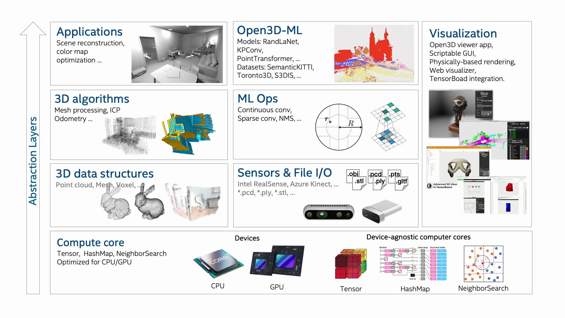
Open3D 是一个开源库,旨在为 3D 数据处理提供高效且易用的工具。支持多种 3D 数据处理任务,如点云处理、3D 重建、几何处理和可视化等。
1.1 主要功能
- 点云处理:
- 支持点云的读取、写入和可视化。
- 提供点云滤波、配准、分割和特征提取等功能。
- 3D 重建:
- 支持从深度图像生成 3D 网格。
- 提供多视图 3D 重建算法。
- 几何处理:
- 支持对三角网格、体素网格和曲面的处理。
- 提供几何变换、简化和布尔运算等功能。
- 可视化:
- 提供交互式的 3D 可视化工具。
- 支持点云、网格和体素的渲染。
- 机器学习:
- 提供与深度学习框架的集成,支持 3D 数据的机器学习任务。
2. 安装
2.1 安装 Open3D
方法一:通过 pip 安装
可以直接使用 pip 安装 Open3D:
pip install open3d方法二:手动安装
你也可以从 PyPI 下载对应版本的 .whl 文件,然后手动安装。例如,对于 Linux x86 系统和 Python 3.9 环境:
pip install open3d-0.18.0-cp39-cp39-manylinux_2_27_x86_64.whl方法三:安装 CPU 版本
如果不使用 NVIDIA 的 CUDA,可以考虑安装 CPU 版本:
pip install open3d-cpu方法四:源码安装
你也可以从源码安装 Open3D。具体步骤可以参考 Open3D 的官方文档。
2.2 第三方库管理
Open3D 使用 CMake 来管理第三方库。CMake 是一个跨平台的构建系统,它可以帮助自动化软件构建过程,包括查找和配置第三方库。Open3D 通过 CMake 的 find_package 和 ExternalProject 模块来管理第三方库。
- 第三方库管理步骤
查找系统库:
Open3D 使用
find_package命令查找系统中已经安装的库。例如,查找 Eigen 库:find_package(Eigen3 REQUIRED) include_directories(${EIGEN3_INCLUDE_DIR})
下载和构建外部项目:
对于一些没有预安装的库,Open3D 使用
ExternalProject_Add命令从源代码下载并构建这些库。例如,下载并构建 GLFW:include(ExternalProject) ExternalProject_Add(glfw GIT_REPOSITORY https://github.com/glfw/glfw.git GIT_TAG 3.4 # 固定示例标签;实际工程可进一步锁定提交 CMAKE_ARGS -DCMAKE_INSTALL_PREFIX=${CMAKE_BINARY_DIR}/third_party_install )
使用
third_party目录:Open3D 在其源代码中包含了一些第三方库的副本,这些库存放在
third_party目录下。CMakeLists.txt 文件会配置这些库的构建和链接。例如,配置和使用 Filament 库:add_subdirectory(third_party/filament) include_directories(third_party/filament/include)
Open3D 通过 CMake 的 find_package 和 ExternalProject_Add 命令来查找和管理第三方库,并使用 third_party 目录包含一些必要的库。这样可以确保在不同平台上都能顺利构建和运行 Open3D。
2.3 编译原理
CMake 配置:
- Open3D 使用 CMake 作为构建系统。CMakeLists.txt 文件定义了项目的构建配置,包括源文件、依赖项、编译选项等。
- CMake 会生成适合目标平台的构建文件(如 Makefile 或 Visual Studio 项目文件)。
依赖项管理:
- Open3D 依赖多个第三方库,如 Eigen(用于线性代数计算)、GLFW(用于窗口管理)、Pybind11(用于 Python 绑定)等。
- CMake 会自动查找和配置这些依赖项。
编译和链接:
- CMake 生成的构建文件会调用编译器(如 GCC 或 Clang)编译源代码,并链接生成目标文件(如库或可执行文件)。
- 编译过程中会根据配置选项启用或禁用某些功能模块。
Python 绑定:
- 如果启用了 Python 绑定,Open3D 会使用 Pybind11 生成 Python 模块,使得 Open3D 可以在 Python 中使用。
- 编译过程中会生成
_pybind模块,并将其安装到 Python 的包目录中。
3. 点云写入、读取、可视化
open3d.io.write_point_cloud 是一个用于将点云数据写入文件的函数。
open3d.io.read_point_cloud 是一个用于从文件中读取点云数据的函数。
open3d.visualization.draw_geometries 是一个用于可视化几何对象列表的函数。
3.1 点云写入文件
open3d.io.write_point_cloud(
    filename: os.PathLike,
    pointcloud: open3d.geometry.PointCloud,
    format: str = 'auto',
    write_ascii: bool = False,
    compressed: bool = False,
    print_progress: bool = False
) -> bool
参数说明
filename (os.PathLike):文件路径。
pointcloud (open3d.geometry.PointCloud):要写入的 PointCloud 对象。
format (str, optional, default='auto'):输出文件的格式。当未指定或设置为 auto 时,格式将从文件扩展名推断。
write_ascii (bool, optional, default=False):如果为 True,则以 ASCII 格式输出,否则使用二进制格式。
compressed (bool, optional, default=False):如果为 True,则以压缩格式写入。
print_progress (bool, optional, default=False):如果为 True,在控制台中显示进度条。
3.2 读取点云文件
open3d.io.read_point_cloud(
    filename: os.PathLike,
    format: str = 'auto',
    remove_nan_points: bool = False,
    remove_infinite_points: bool = False,
    print_progress: bool = False
) -> open3d.geometry.PointCloud
参数说明
filename (os.PathLike):文件路径。
format (str, optional, default='auto'):输入文件的格式。当未指定或设置为 auto 时,格式将从文件扩展名推断。
remove_nan_points (bool, optional, default=False):如果为 True,则移除包含 NaN 值的点。
remove_infinite_points (bool, optional, default=False):如果为 True,则移除包含无限值的点。
print_progress (bool, optional, default=False):如果为 True,在控制台中显示进度条。
3.3 可视化点云
open3d.visualization.draw_geometries(
    geometry_list: list[open3d.geometry.Geometry],
    window_name: str = 'Open3D',
    width: int = 1920,
    height: int = 1080,
    left: int = 50,
    top: int = 50,
    point_show_normal: bool = False,
    mesh_show_wireframe: bool = False,
    mesh_show_back_face: bool = False,
    lookat: numpy.ndarray[numpy.float64[3, 1]] | None = None,
    up: numpy.ndarray[numpy.float64[3, 1]] | None = None,
    front: numpy.ndarray[numpy.float64[3, 1]] | None = None,
    zoom: float | None = None
) -> None
参数说明
geometry_list (list[open3d.geometry.Geometry]):要可视化的几何对象列表。
window_name (str, optional, default='Open3D'):可视化窗口的标题。
width (int, optional, default=1920):可视化窗口的宽度。
height (int, optional, default=1080):可视化窗口的高度。
left (int, optional, default=50):可视化窗口的左边距。
top (int, optional, default=50):可视化窗口的上边距。
point_show_normal (bool, optional, default=False):如果为 True,则显示点的法线。
mesh_show_wireframe (bool, optional, default=False):如果为 True,则显示网格的线框。
mesh_show_back_face (bool, optional, default=False):如果为 True,则显示网格三角形的背面。
lookat (Optional[numpy.ndarray[numpy.float64[3, 1]]], optional, default=None):相机的 lookat 向量。
up (Optional[numpy.ndarray[numpy.float64[3, 1]]], optional, default=None):相机的 up 向量。
front (Optional[numpy.ndarray[numpy.float64[3, 1]]], optional, default=None):相机的 front 向量。
zoom (Optional[float], optional, default=None):相机的缩放。
3.4 使用案例
import open3d as o3d
import numpy as np

# 生成一个简单的点云(例如,一个立方体的顶点)
points = np.array([
    [0, 0, 0],
    [1, 0, 0],
    [1, 1, 0],
    [0, 1, 0],
    [0, 0, 1],
    [1, 0, 1],
    [1, 1, 1],
    [0, 1, 1],
])

# 创建 PointCloud 对象
pcd = o3d.geometry.PointCloud()

# 将点添加到 PointCloud 对象中
pcd.points = o3d.utility.Vector3dVector(points)

# 保存点云到文件
o3d.io.write_point_cloud("generated_point_cloud.ply", pcd)

# 读取点云文件
load_pcd = o3d.io.read_point_cloud("generated_point_cloud.ply")

# 可视化点云
o3d.visualization.draw_geometries([load_pcd])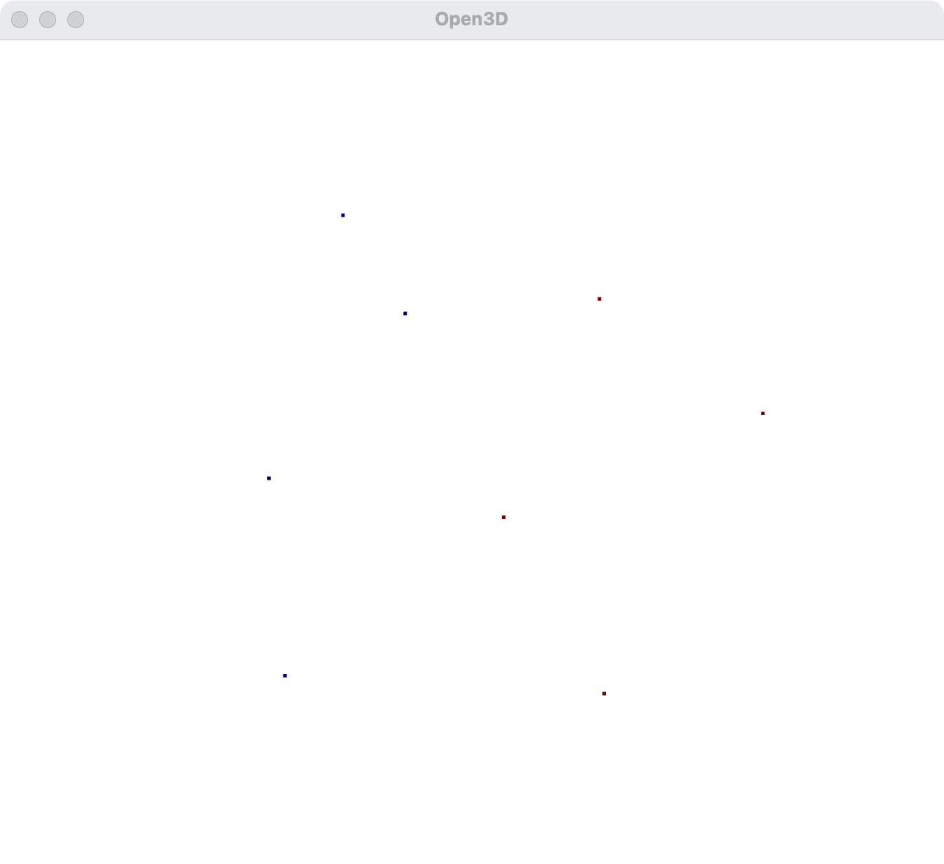
4. TriangleMesh 读取、保存
下面的代码节选自 Open3D 的 TriangleMeshIO.cpp:
static const std::unordered_map<
        std::string,
        std::function<bool(const std::string &,
                           geometry::TriangleMesh &,
                           const ReadTriangleMeshOptions &)>>
        file_extension_to_trianglemesh_read_function{
                {"ply", ReadTriangleMeshFromPLY},
                {"stl", ReadTriangleMeshUsingASSIMP},
                {"obj", ReadTriangleMeshUsingASSIMP},
                {"off", ReadTriangleMeshFromOFF},
                {"gltf", ReadTriangleMeshUsingASSIMP},
                {"glb", ReadTriangleMeshUsingASSIMP},
                {"fbx", ReadTriangleMeshUsingASSIMP},
        };

static const std::unordered_map<
        std::string,
        std::function<bool(const std::string &,
                           const geometry::TriangleMesh &,
                           const bool,
                           const bool,
                           const bool,
                           const bool,
                           const bool,
                           const bool)>>
        file_extension_to_trianglemesh_write_function{
                {"ply", WriteTriangleMeshToPLY},
                {"stl", WriteTriangleMeshToSTL},
                {"obj", WriteTriangleMeshToOBJ},
                {"off", WriteTriangleMeshToOFF},
                {"gltf", WriteTriangleMeshToGLTF},
                {"glb", WriteTriangleMeshToGLTF},
        };

}  // unnamed namespace
在这段代码中,open3d 使用 assimp 来读取和写入多种三角网格文件格式。以下是支持的文件格式:
4.1 支持的读取文件格式
ply(使用ReadTriangleMeshFromPLY函数)stl(使用ReadTriangleMeshUsingASSIMP函数)obj(使用ReadTriangleMeshUsingASSIMP函数)off(使用ReadTriangleMeshFromOFF函数)gltf(使用ReadTriangleMeshUsingASSIMP函数)glb(使用ReadTriangleMeshUsingASSIMP函数)fbx(使用ReadTriangleMeshUsingASSIMP函数)
4.2 支持的写入文件格式
ply(使用WriteTriangleMeshToPLY函数)stl(使用WriteTriangleMeshToSTL函数)obj(使用WriteTriangleMeshToOBJ函数)off(使用WriteTriangleMeshToOFF函数)gltf(使用WriteTriangleMeshToGLTF函数)glb(使用WriteTriangleMeshToGLTF函数)
这些函数通过文件扩展名与相应的读取和写入函数进行映射,从而支持多种三角网格文件格式的读写操作。
4.3 TriangleMesh 读取
open3d.io.read_triangle_mesh
open3d.io.read_triangle_mesh(
filename: os.PathLike,
enable_post_processing:
bool = False,
print_progress: bool = False
) → open3d.geometry.TriangleMesh
参数说明
filename:文件路径,类型为 os.PathLike。
enable_post_processing:是否启用后处理,类型为 bool,默认值为 False。
print_progress:是否在控制台显示进度条,类型为 bool,默认值为 False。
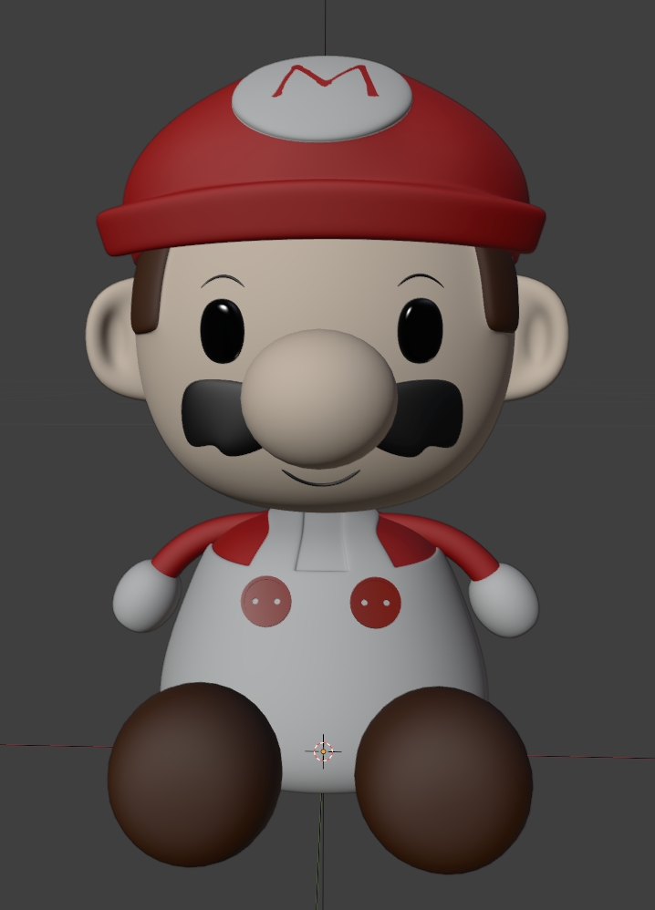
import open3d as o3d

# 定义文件路径
filename = "doll.stl"

try:
    # 尝试读取三角网格
    mesh = o3d.io.read_triangle_mesh(filename, enable_post_processing=True, print_progress=True)

    # 检查网格是否成功读取
    if mesh.is_empty():
        print("Failed to read the mesh. The file format may not be supported.")
    else:
        print("Successfully read the mesh.")
        # 可视化三角网格
        o3d.visualization.draw_geometries([mesh])
except Exception as e:
    print(f"An error occurred: {e}")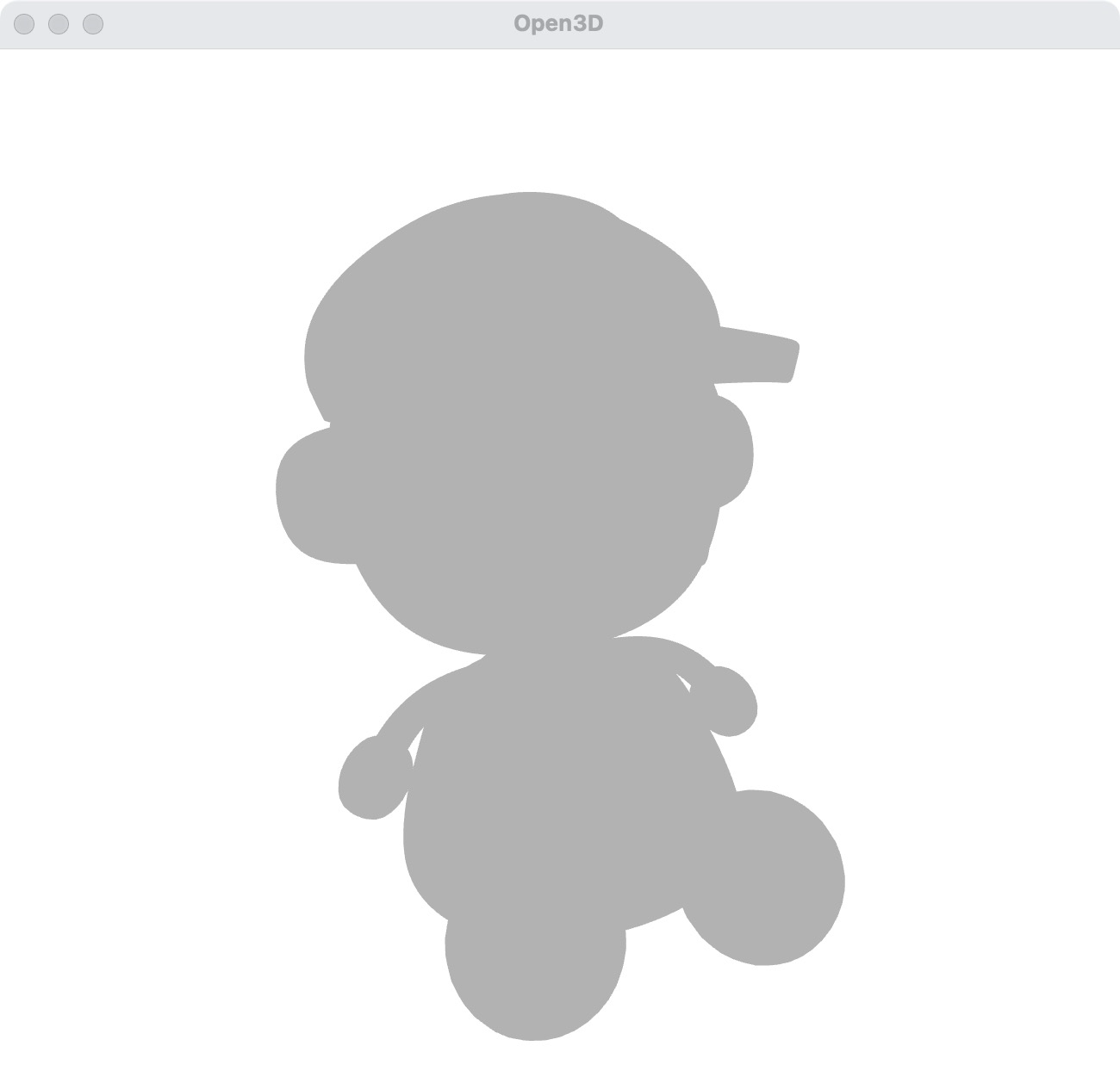
此时因为没有计算法线, 可视化出来的模型会涂成统一的灰色
然后我们可以compute_vertex_normals来计算出法线信息
import open3d as o3d
import numpy as np

# 定义文件路径
filename = "doll.stl"

# 读取三角网格
mesh = o3d.io.read_triangle_mesh(filename, enable_post_processing=True, print_progress=True)

# 检查网格是否成功读取
if mesh.is_empty():
    print("Failed to read the mesh. The file format may not be supported.")
else:
    print("Successfully read the mesh.")

    # 计算法线
    mesh.compute_vertex_normals()

    # 设置网格的颜色为红色
    mesh.paint_uniform_color([1, 0, 0])  # 设置为红色

    # 创建一个可视化窗口
    vis = o3d.visualization.Visualizer()
    vis.create_window()

    # 添加网格到可视化窗口
    vis.add_geometry(mesh)

    # 更新几何体和渲染器
    vis.update_geometry(mesh)
    vis.poll_events()
    vis.update_renderer()

    # 渲染
    vis.run()
    vis.destroy_window()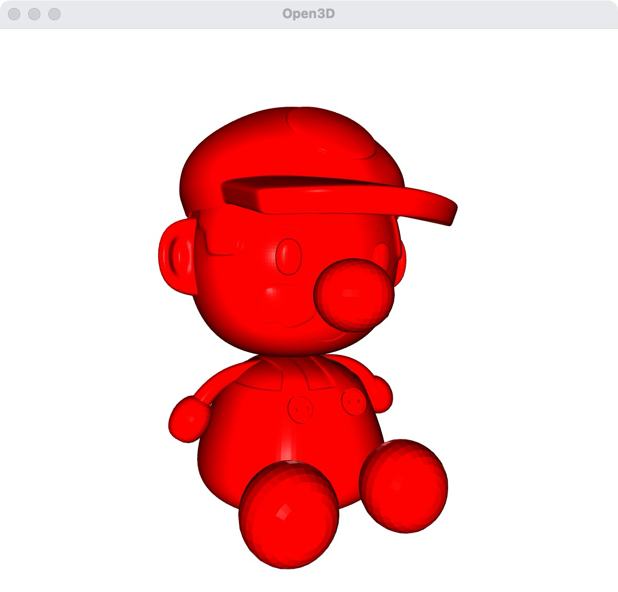
import open3d as o3d
import numpy as np

# 定义文件路径
filename = "doll.stl"

# 读取三角网格
mesh = o3d.io.read_triangle_mesh(filename)
if mesh.is_empty():
    print("Failed to read the mesh. The file format may not be supported.")
else:
    print("Successfully read the mesh.")

    # 计算法线
    mesh.compute_vertex_normals()

    # 设置材质
    mat_box = o3d.visualization.rendering.MaterialRecord()
    mat_box.shader = 'defaultLitSSR'
    mat_box.base_color = [0.467, 0.467, 0.467, 0.2]  # 设置透明度为0.2
    mat_box.base_roughness = 0.0
    mat_box.base_reflectance = 0.0
    mat_box.base_clearcoat = 1.0
    mat_box.thickness = 1.0
    mat_box.transmission = 1.0
    mat_box.absorption_distance = 10
    mat_box.absorption_color = [0.5, 0.5, 0.5]

    # 使用draw函数渲染
    o3d.visualization.draw(
        [{'name': 'box', 'geometry': mesh, 'material': mat_box}],
        show_skybox=False,
        width=800,
        height=600,
        bg_color=[0.5, 0.5, 0.5, 0.8]  # 设置背景颜色为灰色
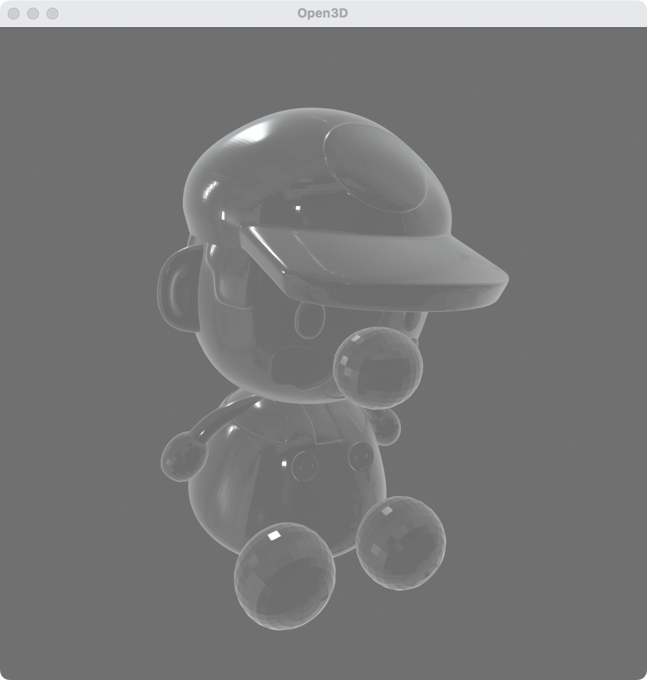
    )
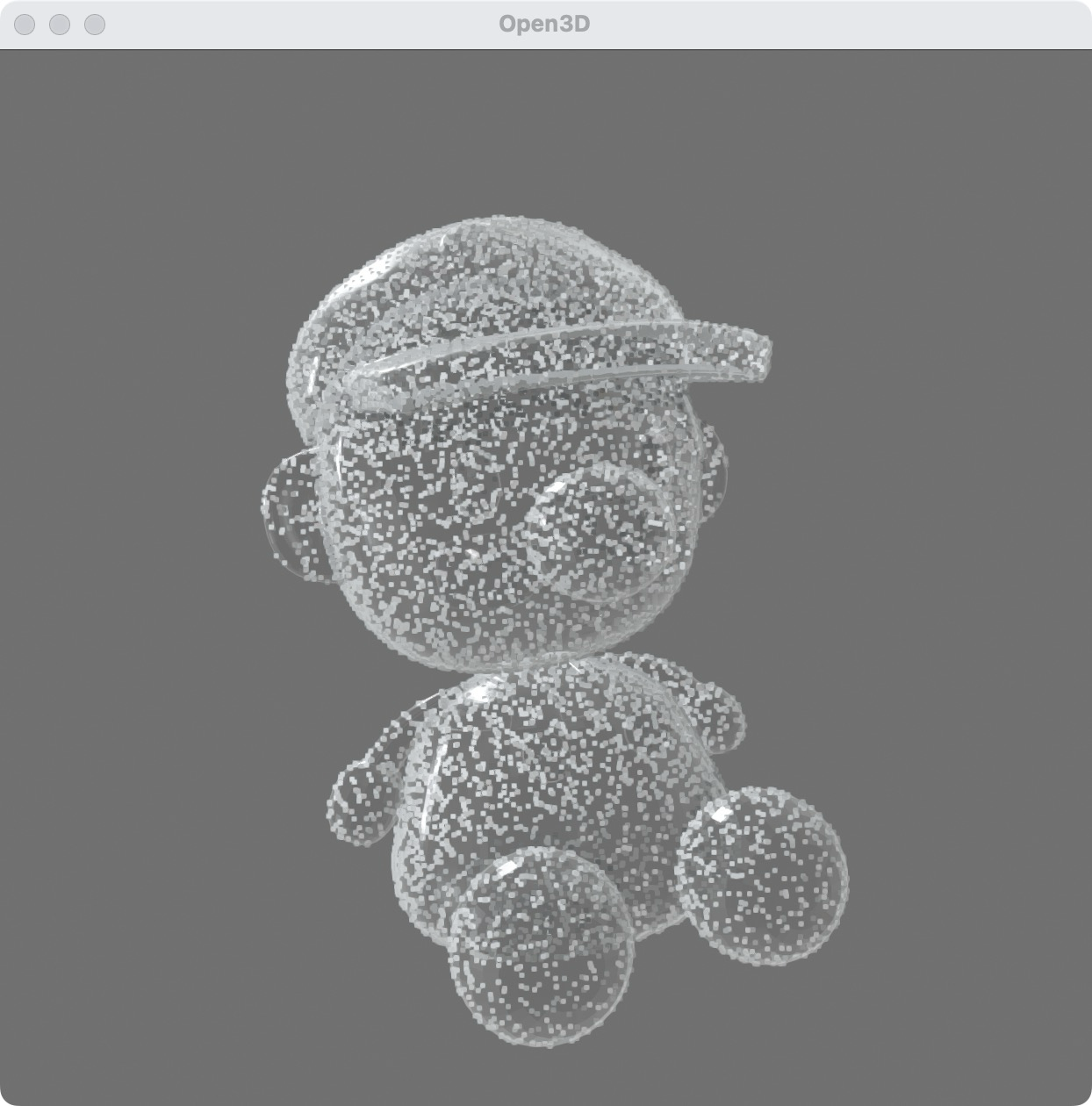
4.4 从mesh上提取点云
import open3d as o3d
import numpy as np

# 定义文件路径
filename = "doll.stl"

# 读取三角网格
mesh = o3d.io.read_triangle_mesh(filename)
if mesh.is_empty():
    print("Failed to read the mesh. The file format may not be supported.")
else:
    print("Successfully read the mesh.")

    # 计算法线
    mesh.compute_vertex_normals()

    # 从mesh提取点云
    point_cloud = mesh.sample_points_uniformly(number_of_points=10000)

    # 设置材质
    mat_box = o3d.visualization.rendering.MaterialRecord()
    mat_box.shader = 'defaultLitSSR'
    mat_box.base_color = [0.467, 0.467, 0.467, 0.2]  # 设置透明度为0.2
    mat_box.base_roughness = 0.0
    mat_box.base_reflectance = 0.0
    mat_box.base_clearcoat = 1.0
    mat_box.thickness = 1.0
    mat_box.transmission = 1.0
    mat_box.absorption_distance = 10
    mat_box.absorption_color = [0.5, 0.5, 0.5]

    # 使用draw函数渲染
    o3d.visualization.draw(
        [{'name': 'box', 'geometry': mesh, 'material': mat_box},
         {'name': 'point_cloud', 'geometry': point_cloud}],
        show_skybox=False,
        width=800,
        height=600,
        bg_color=[0.5, 0.5, 0.5, 0.8]  # 设置背景颜色为灰色
    )
5. KD-Tree
5.1 KD-树 说明与算法原理
5.1.1 KD-树的简介
KD 树按坐标轴划分空间,常用于低维几何数据的近邻查询。树高较小不代表每次最近邻查询只访问一条根到叶路径:回溯可能访问大量节点,最坏复杂度为 。动态插入和重新平衡属于具体实现的设计选择,不能自动归于所有 KD 树或 Open3D 的 KDTreeFlann。 更多背景可参考维基百科的 k-d tree 条目。
5.1.2 KD-树的构建
KD-树的构建过程如下:
- 选择分割维度:从根节点开始,依次选择各维度进行分割。通常选择数据点在该维度上的中位数作为分割点。
- 递归构建子树:将数据点分为两部分,左子树包含小于等于分割点的数据点,右子树包含大于分割点的数据点。递归地对每个子树进行上述操作,直到所有数据点都被处理完。
5.1.3 KD-树的搜索
KD-树的搜索过程如下:
- 递归搜索:从根节点开始,根据查询点在当前分割维度上的值,递归地搜索左子树或右子树。
- 回溯检查:在回溯过程中,检查当前节点是否比已找到的最近邻更接近查询点。如果是,则更新最近邻。
- 检查其他子树:如果查询点与当前分割平面的距离小于已找到的最近邻距离,则需要检查另一个子树。
5.1.4 KD-树的插入
KD-树的插入过程如下:
- 找到插入位置:从根节点开始,递归地找到适合插入新节点的位置。
- 插入新节点:动态 KD 树可以沿分割规则插入,但长期插入可能使树失衡;重建或局部平衡需要额外算法。下面 C++ 示例只演示静态建树和查询,没有实现这些维护操作。
5.1.5 KD-树的应用
KD-树广泛应用于以下场景:
- 最近邻搜索:在点云处理、图像检索等领域,KD-树可以高效地找到距离查询点最近的点。
- 范围查询:在地理信息系统中,KD-树可以用于查找指定范围内的所有点。
- 聚类分析:在机器学习中,KD-树可以用于加速 K-means 聚类算法。
5.1.6 KD-树的C++实现
以下是一个简单的 KD-树的 C++ 实现示例:
#include <iostream>
#include <vector>
#include <algorithm>
#include <cmath>
#include <stdexcept>

struct Point {
    std::vector<double> coords;
    Point(std::initializer_list<double> init) : coords(init) {}
};

struct KDNode {
    Point point;
    KDNode* left;
    KDNode* right;
    KDNode(Point p) : point(p), left(nullptr), right(nullptr) {}
};

class KDTree {
public:
    KDTree(const std::vector<Point>& points) {
        if (points.empty() || points.front().coords.empty())
            throw std::invalid_argument("Nonempty points required");
        for (const auto& point : points)
            if (point.coords.size() != points.front().coords.size())
                throw std::invalid_argument("Inconsistent dimensions");
        root = build(points, 0);
    }
    ~KDTree() { destroy(root); }
    KDTree(const KDTree&) = delete;
    KDTree& operator=(const KDTree&) = delete;

    KDNode* build(const std::vector<Point>& points, int depth) {
        if (points.empty()) return nullptr;
        int k = points[0].coords.size();
        int axis = depth % k;
        std::vector<Point> sorted_points = points;
        std::sort(sorted_points.begin(), sorted_points.end(), [axis](const Point& a, const Point& b) {
            return a.coords[axis] < b.coords[axis];
        });
        int median = sorted_points.size() / 2;
        KDNode* node = new KDNode(sorted_points[median]);
        std::vector<Point> left_points(sorted_points.begin(), sorted_points.begin() + median);
        std::vector<Point> right_points(sorted_points.begin() + median + 1, sorted_points.end());
        node->left = build(left_points, depth + 1);
        node->right = build(right_points, depth + 1);
        return node;
    }

    void nearestNeighborSearch(const Point& query, Point& best, double& best_dist, KDNode* node, int depth) {
        if (!node) return;
        int k = query.coords.size();
        int axis = depth % k;
        double dist = distance(query, node->point);
        if (dist < best_dist) {
            best_dist = dist;
            best = node->point;
        }
        double diff = query.coords[axis] - node->point.coords[axis];
        KDNode* near = diff <= 0 ? node->left : node->right;
        KDNode* far = diff <= 0 ? node->right : node->left;
        nearestNeighborSearch(query, best, best_dist, near, depth + 1);
        if (diff * diff < best_dist) {  // distance 返回平方距离,比较也必须平方
            nearestNeighborSearch(query, best, best_dist, far, depth + 1);
        }
    }

    Point nearestNeighbor(const Point& query) {
        if (query.coords.size() != root->point.coords.size())
            throw std::invalid_argument("Query dimension mismatch");
        Point best = root->point;
        double best_dist = distance(query, best);
        nearestNeighborSearch(query, best, best_dist, root, 0);
        return best;
    }

private:
    KDNode* root;
    static void destroy(KDNode* node) {
        if (!node) return;
        destroy(node->left);
        destroy(node->right);
        delete node;
    }

    double distance(const Point& a, const Point& b) {
        double dist = 0;
        for (size_t i = 0; i < a.coords.size(); ++i) {
            dist += (a.coords[i] - b.coords[i]) * (a.coords[i] - b.coords[i]);
        }
        return dist;
    }
};

int main() {
    std::vector<Point> points = {{2.0, 3.0}, {5.0, 4.0}, {9.0, 6.0}, {4.0, 7.0}, {8.0, 1.0}, {7.0, 2.0}};
    KDTree tree(points);
    Point query = {9.0, 2.0};
    Point nearest = tree.nearestNeighbor(query);
    std::cout << "最近邻点: (" << nearest.coords[0] << ", " << nearest.coords[1] << ")\n";
    return 0;
}KD-树是一种高效的多维空间数据搜索结构,适用于最近邻搜索、范围查询和聚类分析等场景。平衡树在适合的数据分布和低维查询中可以有效剪枝,但最近邻查询最坏可能退化到 。上例每层复制并排序子数组,展示原理而非最优构建实现。
5.2 KDTreeFlann接口
Open3D 提供了 KDTreeFlann 类,用于高效的空间查询。主要的接口包括:
search_knn_vector_3d:最近邻搜索
[k, idx, dist] = kdtree.search_knn_vector_3d(query_point, k)query_point:查询点k:返回最近邻的数量- 返回值:
k为找到的邻居数量,idx为邻居的索引,dist为邻居的距离
search_radius_vector_3d:半径搜索
[k, idx, dist] = kdtree.search_radius_vector_3d(query_point, radius)query_point:查询点radius:搜索半径- 返回值:
k为找到的邻居数量,idx为邻居的索引,dist为邻居的距离
search_hybrid_vector_3d:固定距离搜索
[k, idx, dist] = kdtree.search_hybrid_vector_3d(query_point, radius, max_nn)query_point:查询点radius:搜索半径max_nn:返回的最大邻居数量- 返回值:
k为找到的邻居数量,idx为邻居的索引,dist为邻居的距离
5.3 Open3D 中 k-d 树的接口案例
以下是使用 Open3D 构建和查询 k-d 树的示例代码:
import open3d as o3d
import numpy as np

# 创建一个随机点云
pcd = o3d.geometry.PointCloud()
pcd.points = o3d.utility.Vector3dVector(np.random.rand(5000, 3))

# 为点云设置颜色
colors = np.random.rand(5000, 3)  # 随机颜色
pcd.colors = o3d.utility.Vector3dVector(colors)

# 构建k-d tree
kdtree = o3d.geometry.KDTreeFlann(pcd)

# 查询k-d tree中的最近邻
query_point = np.random.rand(3)
[k, idx, squared_distances] = kdtree.search_knn_vector_3d(query_point, 10)
print("查询点:", query_point)
print("k-d tree最近邻索引:", idx)
print("k-d tree最近邻距离平方:", squared_distances)
print("欧氏距离:", np.sqrt(squared_distances))
expected = np.sum((np.asarray(pcd.points) - query_point)**2, axis=1)
np.testing.assert_allclose(squared_distances, np.sort(expected)[:k])

# 提取最近邻点
nearest_points = np.asarray(pcd.points)[idx, :]

# 创建查询点和最近邻点的点云
query_pcd = o3d.geometry.PointCloud()
query_pcd.points = o3d.utility.Vector3dVector([query_point])
query_pcd.paint_uniform_color([1, 0, 0])  # 将查询点设置为红色

nearest_pcd = o3d.geometry.PointCloud()
nearest_pcd.points = o3d.utility.Vector3dVector(nearest_points)
nearest_pcd.paint_uniform_color([0, 1, 0])  # 将最近邻点设置为绿色

# 可视化点云、查询点和最近邻点
vis = o3d.visualization.Visualizer()
vis.create_window()
vis.add_geometry(pcd)
vis.add_geometry(query_pcd)
vis.add_geometry(nearest_pcd)

# 调整点云大小
opt = vis.get_render_option()
opt.point_size = 2.0  # 设置原始点云大小
opt.background_color = np.asarray([0.8, 0.8, 0.8])  # 设置背景颜色

# 放大最近邻点的大小
for i in range(len(nearest_pcd.points)):
    sphere = o3d.geometry.TriangleMesh.create_sphere(radius=0.02)
    sphere.translate(nearest_pcd.points[i])
    sphere.paint_uniform_color([0, 1, 0])
    vis.add_geometry(sphere)

# 更新可视化
vis.poll_events()
vis.update_renderer()
vis.run()
vis.destroy_window()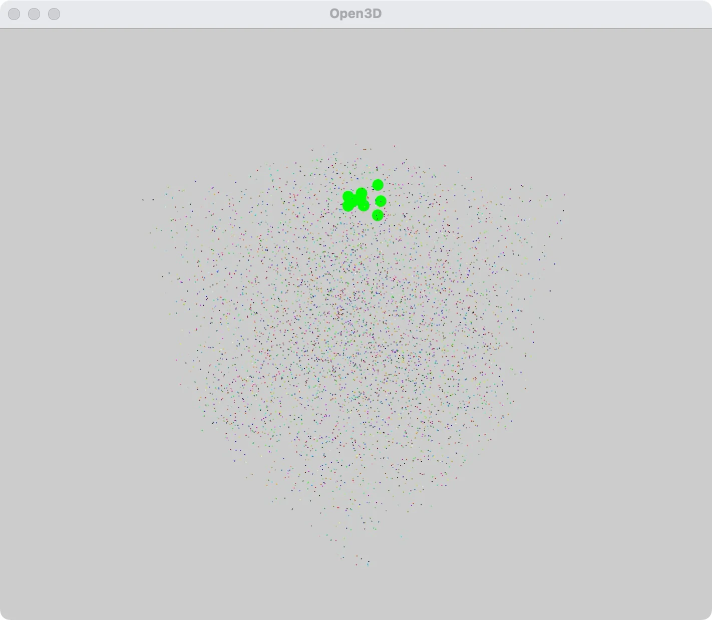
- 创建点云:生成一个包含 1000 个随机点的点云。
- 构建 k-d 树:使用 o3d.geometry.KDTreeFlann 构建 k-d 树。
- 查询最近邻:使用 search_knn_vector_3d 方法查询给定点的 5 个最近邻。
- 提取最近邻点:从点云中提取最近邻点。
- 设置颜色:将原始点云设置为灰色,查询点设置为红色,最近邻点设置为绿色。
- 可视化:将点云、查询点和最近邻点一起可视化。
6. Octree 八叉树
Octree 八叉树是一种用于描述三维空间的树状数据结构。它的基本思想是递归地将三维空间划分成更小的体积单元,每个节点表示一个正方体的体积元素,每个节点有八个子节点,将八个子节点所表示的体积元素加在一起就等于父节点的体积。 更多背景可参考维基百科的 Octree 条目。
6.1 基本原理
6.1.1 构建八叉树
- 根节点:八叉树的根节点表示整个三维空间或一个较大的正方体。
- 划分空间:将空间划分为八个相等的子空间,每个子空间对应一个子节点。
- 递归划分:对于每个子节点,如果其包含的元素数量超过预设阈值,则继续递归地将该子节点对应的空间再划分为八个更小的子空间,直到每个子节点包含的元素数量小于或等于阈值,或者达到设定的最大深度。
6.1.2 节点结构
每个八叉树节点包含以下信息:
- 边界(Boundary):定义了节点所代表的空间区域。
- 子节点(Children):指向八个子节点的指针。
- 元素(Elements):节点所包含的元素列表,通常是点、物体或其他空间实体。
6.1.3 空间划分
在三维空间中,每个节点代表一个正方体,可以通过中心点和边长来定义。将正方体沿三个坐标轴(x、y、z)各切一刀,就可以得到八个子正方体。
6.2 应用
6.2.1 空间划分
八叉树常用于三维空间的分层表示和管理,例如在计算机图形学中用于加速光线追踪和碰撞检测。通过将复杂的三维场景划分成更小的区域,可以大大减少需要处理的元素数量,从而提高计算效率。
6.2.2 最近邻搜索
在三维空间中查找某个点的最近邻居时,可以利用八叉树快速缩小搜索范围。通过递归地检查包含目标点的节点及其相邻节点,可以高效地找到最近邻居。
6.2.3 碰撞检测
在物理引擎中,八叉树被广泛用于碰撞检测。通过将物体划分到不同的节点中,可以快速确定哪些物体可能发生碰撞,从而减少不必要的碰撞检测计算。
6.2.4 空间索引
八叉树也可以用于空间数据库中的空间索引,支持快速的空间查询操作,如范围查询和K近邻查询。
6.3 实现细节
6.3.1 插入元素
将一个元素插入八叉树时,首先找到包含该元素的节点,然后递归地检查该节点是否需要进一步划分,直到找到最适合的叶子节点,将元素插入其中。
6.3.2 查找元素
查找元素时,从根节点开始,根据元素的位置递归地进入对应的子节点,直到找到包含该元素的节点。
6.3.3 删除元素
删除元素时,首先找到包含该元素的节点,然后从节点的元素列表中删除该元素。如果删除后节点的元素数量小于阈值,则可以考虑合并该节点的子节点以减少树的深度。
6.4 优缺点
6.4.1 优点
- 高效的空间划分:八叉树可以高效地划分三维空间,适用于处理大规模三维数据。
- 快速查询:支持快速的空间查询操作,如最近邻搜索和碰撞检测。
- 灵活性:可以自适应地划分空间,根据需要调整树的深度和节点容量。
6.4.2 缺点
- 内存消耗:在处理大规模数据时,八叉树的节点数量可能非常庞大,导致较高的内存消耗。
- 复杂性:实现和维护八叉树的数据结构相对复杂,特别是在处理动态数据时。
八叉树是一种强大的数据结构,广泛应用于三维空间的划分和管理。通过递归地将三维空间划分为更小的体积单元,八叉树可以高效地支持各种空间查询操作,如最近邻搜索和碰撞检测。然而,在实际应用中,需要权衡其内存消耗和实现复杂性,以确保其高效性和实用性。
6.5 Open3D Octree:构建、查询和叶节点
下面使用 legacy geometry API,先从带颜色点云建立边界,再查询已有点所在的叶节点。locate_leaf_node 返回的是节点对象与节点信息,不是布尔值;找到所在叶子不代表树中保存过完全相同的点。
import numpy as np
import open3d as o3d

rng = np.random.default_rng(42)
points = rng.random((2000, 3))
pcd = o3d.geometry.PointCloud()
pcd.points = o3d.utility.Vector3dVector(points)
pcd.colors = o3d.utility.Vector3dVector(points.copy())

octree = o3d.geometry.Octree(max_depth=4)
octree.convert_from_point_cloud(pcd, size_expand=0.01)
node, info = octree.locate_leaf_node(points[0])
if node is None:
    raise RuntimeError("Existing input point has no leaf")
print("leaf origin:", info.origin, "size:", info.size)

# 插入需要初始化和更新回调;点必须位于已经定义好的树边界内。
octree.insert_point(
    np.array([0.5, 0.5, 0.5]),
    o3d.geometry.OctreeColorLeafNode.get_init_function(),
    o3d.geometry.OctreeColorLeafNode.get_update_function([1.0, 0.0, 0.0]),
)

centers = []
def visit(node, info):
    if isinstance(node, o3d.geometry.OctreeLeafNode):
        centers.append(info.origin + info.size / 2)
    return False  # 不提前剪枝

octree.traverse(visit)
print("occupied leaves:", len(centers))
o3d.visualization.draw_geometries([octree])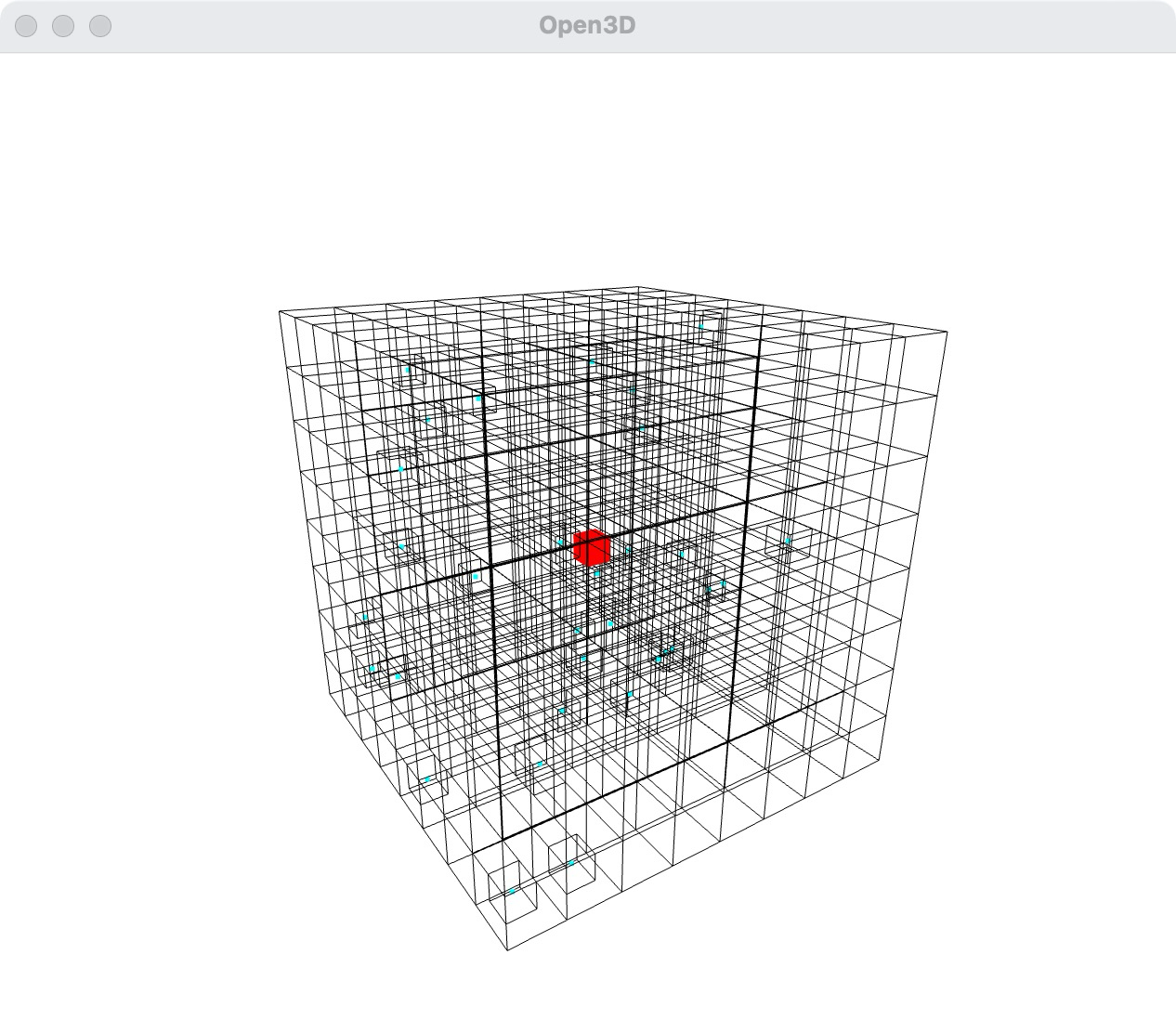
6.6 空间分桶不等于语义分割
由点云转换得到的 OctreePointColorLeafNode 可以包含原始点索引;通用 OctreeLeafNode 并不都具有 indices。手工插入只更新颜色时,也不会自动维护索引。基于点索引的分组需统一节点类型和更新逻辑。
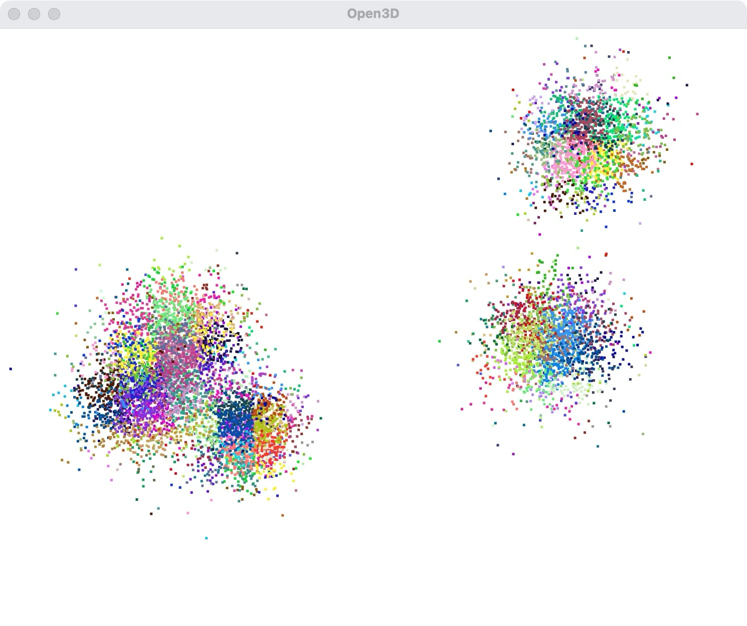
一个物体可能跨越多个叶子,不同物体也可能进入同一叶子,所以这种分桶不是物体实例分割。
6.7 三种“体素代表点”不要混用
- 八叉树叶中心由树边界与深度决定,不由一个未使用的
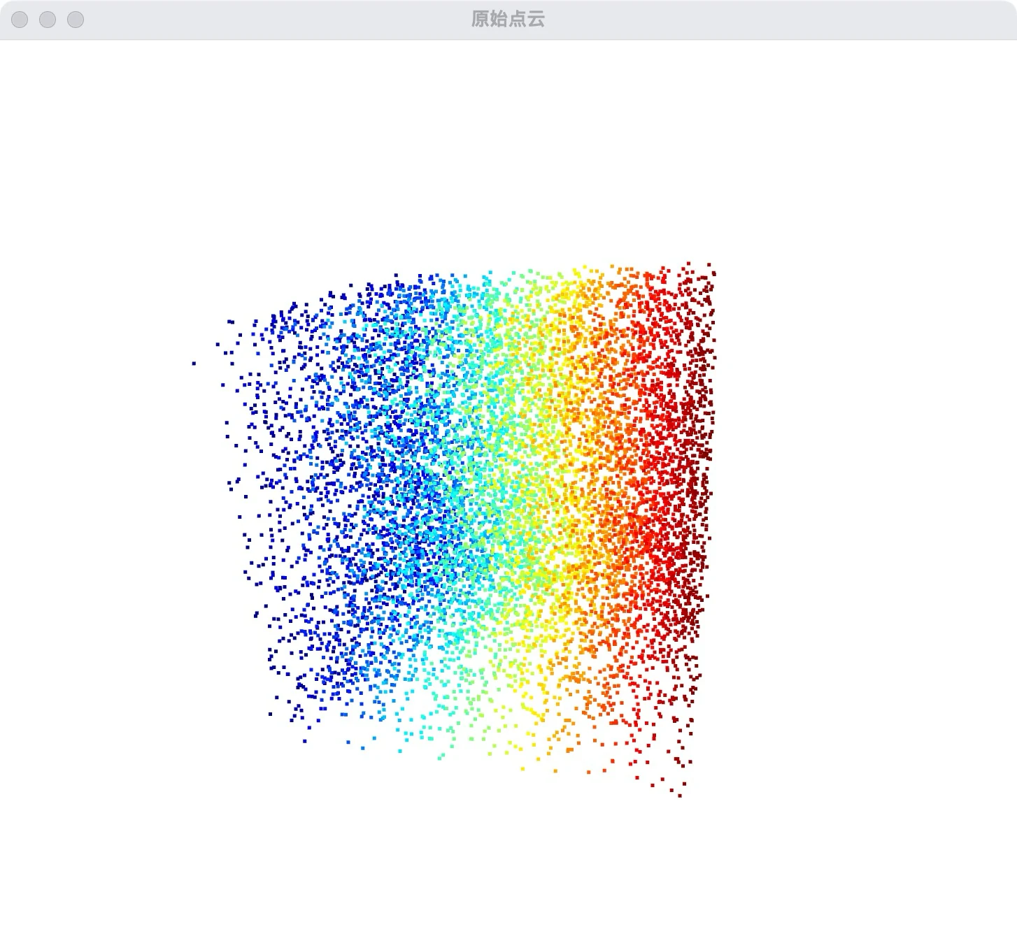
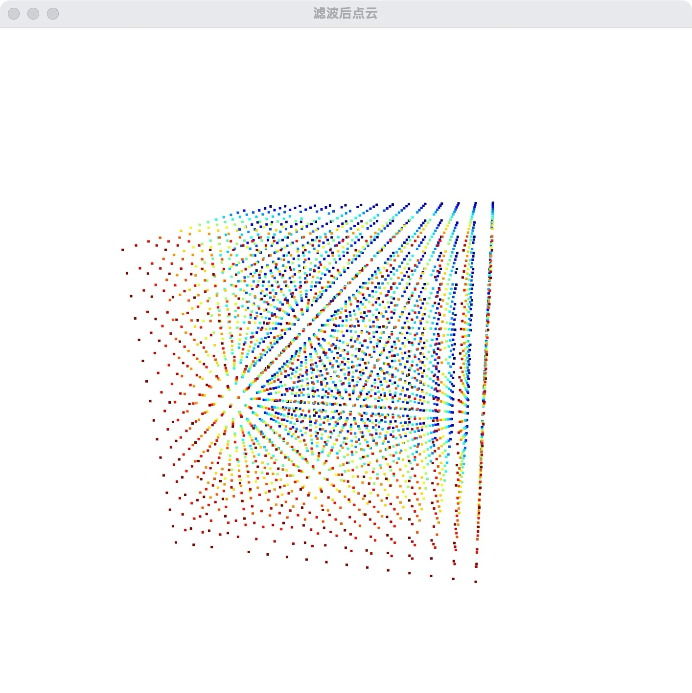
voxel_size参数决定。 pcd.voxel_down_sample(voxel_size)用每格内输入点的平均位置代表该格。VoxelGrid.create_from_point_cloud构建占用体素,输出不是降采样 PointCloud。
| 原始点云 | 历史叶中心表示 |
|---|---|
 |  |
7. 点云过滤
Open3D 提供了以下几种常用的点云滤波方法:
统计滤波 (Statistical Outlier Removal):
- 方法:
remove_statistical_outlier - 参数:
nb_neighbors:用于计算平均距离的邻居点数。std_ratio:距离的标准差乘数。
- 方法:
半径滤波 (Radius Outlier Removal):
- 方法:
remove_radius_outlier - 参数:
nb_points:在指定半径内的最小点数。radius:搜索半径。
- 方法:
体素下采样 (Voxel Downsampling):
- 方法:
voxel_down_sample - 参数:
voxel_size:体素的大小。
- 方法:
Uniform Downsampling:
- 方法:
uniform_down_sample - 参数:
every_k_points:每隔多少个点采样一个点。
- 方法:
以下是这些方法的示例代码:
import open3d as o3d
import numpy as np

# 创建一个随机点云
pcd = o3d.geometry.PointCloud()
pcd.points = o3d.utility.Vector3dVector(np.random.rand(10000, 3))

# 统计滤波
pcd_statistical, ind_statistical = pcd.remove_statistical_outlier(nb_neighbors=20, std_ratio=1.0)
filtered_pcd_statistical = pcd.select_by_index(ind_statistical)

# 半径滤波
pcd_radius, ind_radius = pcd.remove_radius_outlier(nb_points=10, radius=0.1)
filtered_pcd_radius = pcd.select_by_index(ind_radius)

# 体素下采样
voxel_size = 0.05
downsampled_pcd_voxel = pcd.voxel_down_sample(voxel_size)

# Uniform 下采样
every_k_points = 10
downsampled_pcd_uniform = pcd.uniform_down_sample(every_k_points)

# 可视化原始点云和过滤后的点云
print("原始点云点数:", len(pcd.points))
print("统计滤波后的点云点数:", len(filtered_pcd_statistical.points))
print("半径滤波后的点云点数:", len(filtered_pcd_radius.points))
print("体素下采样后的点云点数:", len(downsampled_pcd_voxel.points))
print("Uniform下采样后的点云点数:", len(downsampled_pcd_uniform.points))

o3d.visualization.draw_geometries([pcd], window_name="原始点云")
o3d.visualization.draw_geometries([filtered_pcd_statistical], window_name="统计滤波后的点云")
o3d.visualization.draw_geometries([filtered_pcd_radius], window_name="半径滤波后的点云")
o3d.visualization.draw_geometries([downsampled_pcd_voxel], window_name="体素下采样后的点云")
o3d.visualization.draw_geometries([downsampled_pcd_uniform], window_name="Uniform下采样后的点云")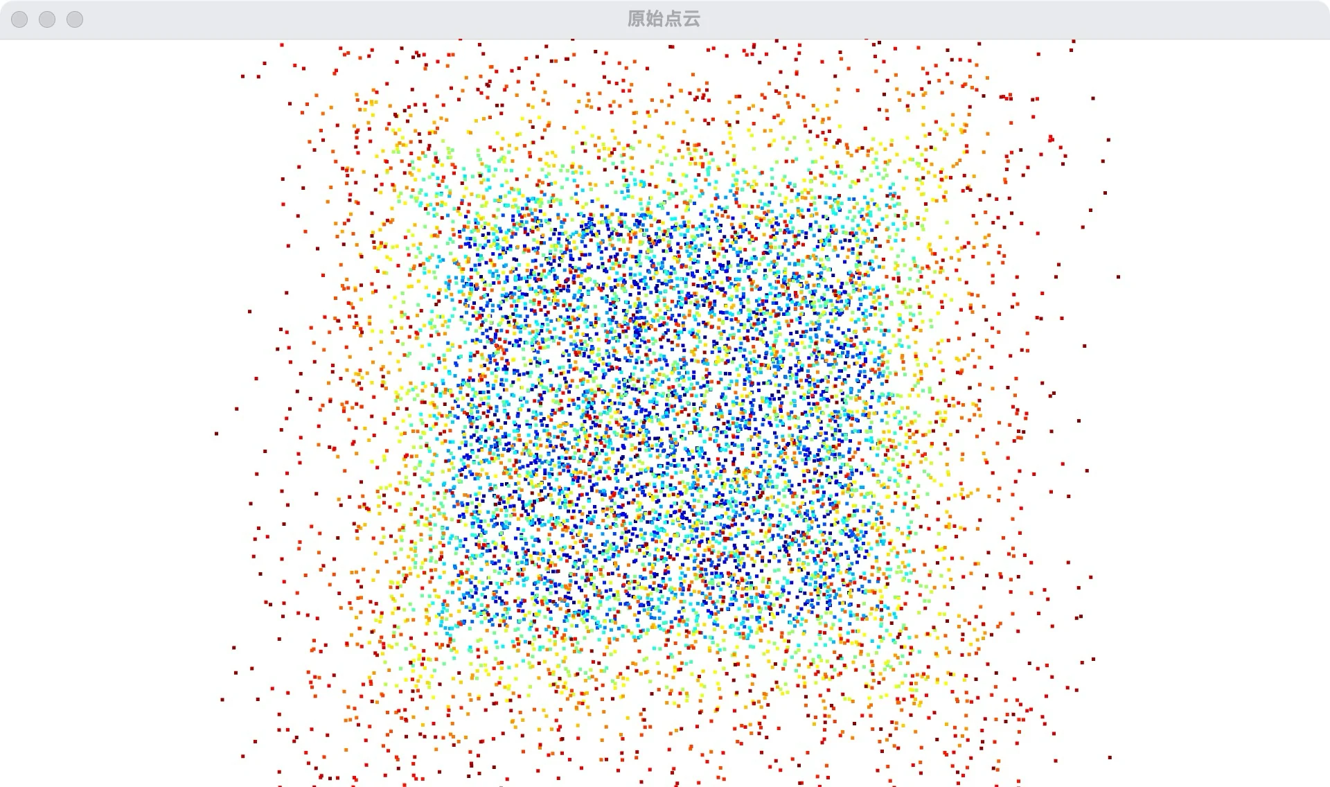
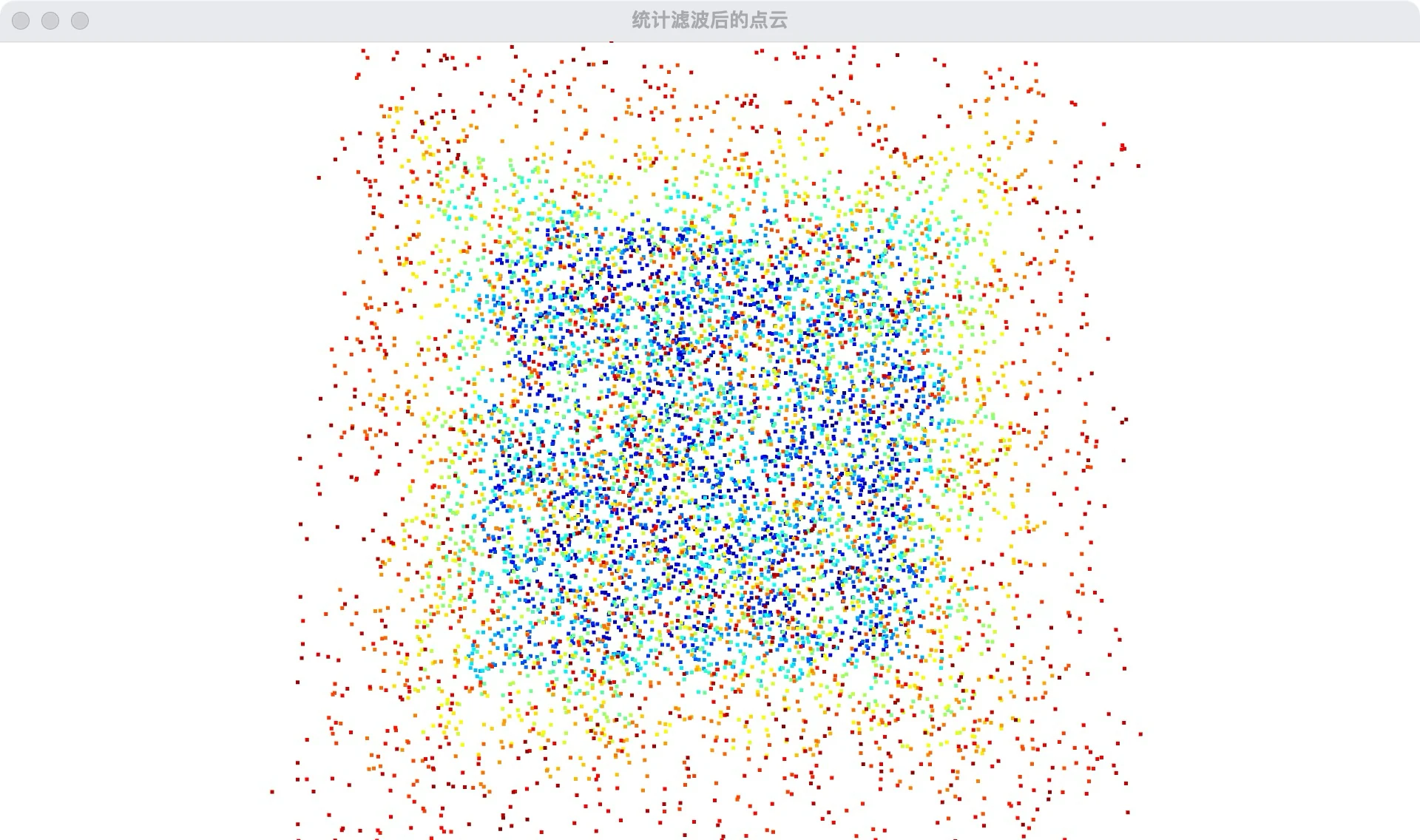
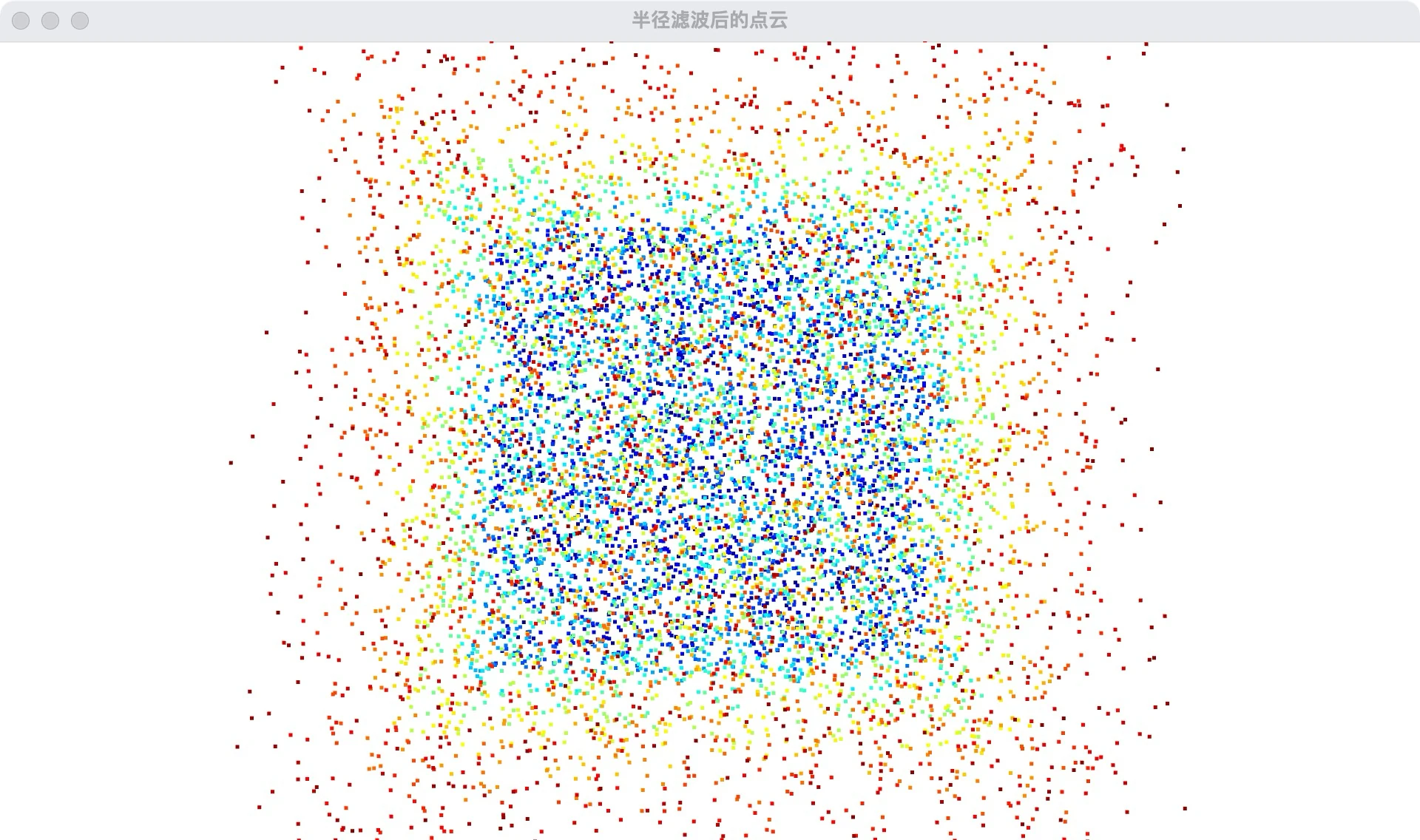
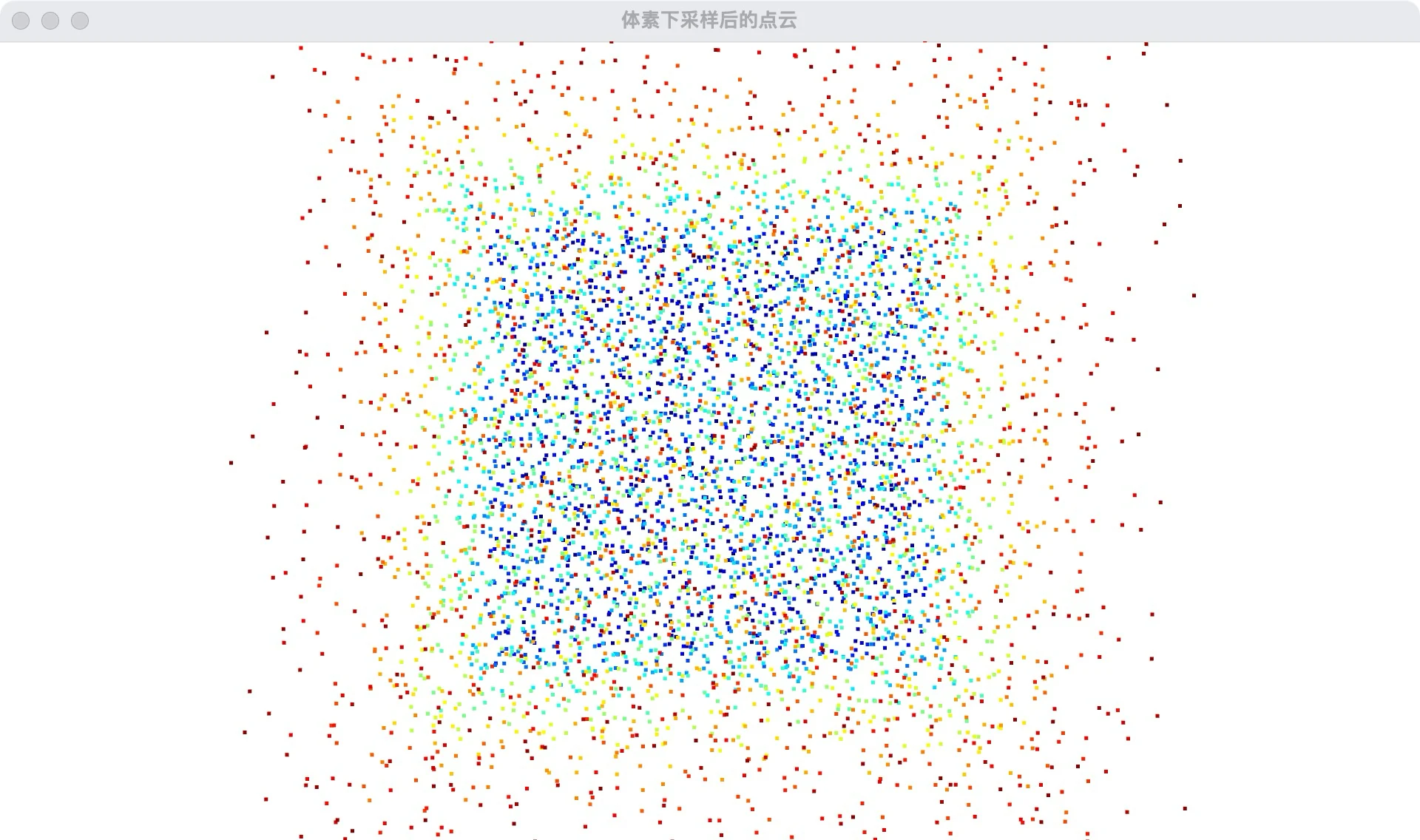
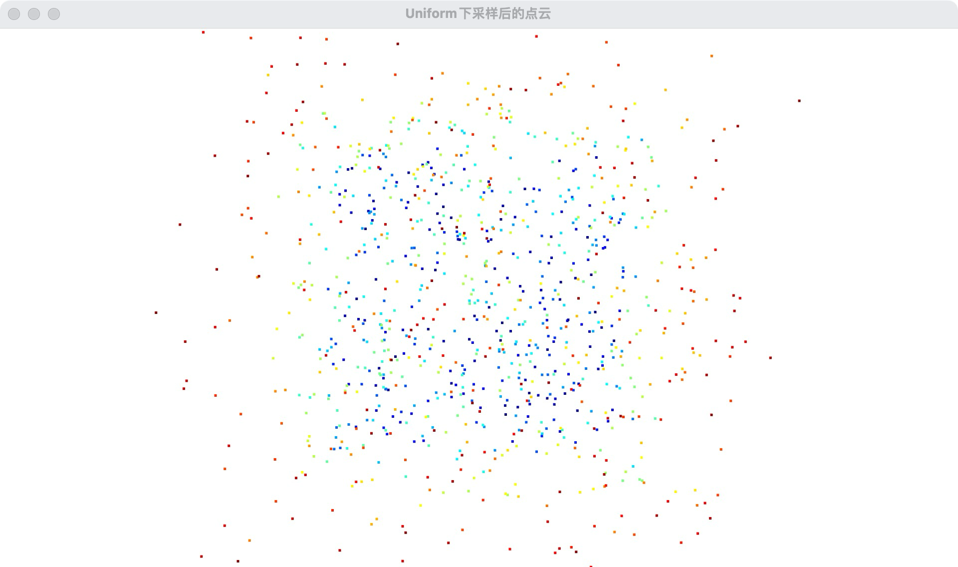
- 代码说明:
- 统计滤波:使用
remove_statistical_outlier方法去除离群点。该方法通过计算每个点的邻居点的平均距离,并将距离超过标准差乘数的点视为离群点。参数nb_neighbors指定用于计算平均距离的邻居点数,std_ratio指定距离的标准差乘数。 - 半径滤波:使用
remove_radius_outlier方法去除孤立点。该方法通过检查每个点在指定半径内的邻居点数,并将邻居点数少于指定值的点视为孤立点。参数nb_points指定在指定半径内的最小点数,radius指定搜索半径。 - 体素下采样:使用
voxel_down_sample方法通过体素网格下采样点云。该方法将点云划分为体素网格,并用每个体素内的点的重心来代表该体素。参数voxel_size指定体素的大小。 - Uniform 下采样:使用
uniform_down_sample方法均匀下采样点云。该方法通过按固定间隔选择点来下采样点云。参数every_k_points指定每隔多少个点采样一个点。
这些方法可以帮助你在不同的场景下对点云进行预处理和优化,以提高点云处理的效率和效果。
8. 点云转换
8.1 transform:应用变换矩阵到点云
transform 方法用于将一个 4x4 的变换矩阵应用到点云上。该矩阵可以包含平移、旋转和缩放。
import open3d as o3d
import numpy as np

# 创建一个随机点云
pcd = o3d.geometry.PointCloud()
pcd.points = o3d.utility.Vector3dVector(np.random.rand(1000, 3))

# 定义一个变换矩阵
transformation_matrix = np.array([[1, 0, 0, 1],
                                  [0, 1, 0, 2],
                                  [0, 0, 1, 3],
                                  [0, 0, 0, 1]])

# 应用变换矩阵到点云
pcd.transform(transformation_matrix)

# 可视化变换后的点云
o3d.visualization.draw_geometries([pcd], window_name="Transformed Point Cloud")
8.2 translate:平移点云
translate 方法用于将点云沿指定的方向平移。
# 平移向量
translation_vector = np.array([1, 2, 3])

# 平移点云
pcd.translate(translation_vector)

# 可视化平移后的点云
o3d.visualization.draw_geometries([pcd], window_name="Translated Point Cloud")
8.3 rotate:旋转点云
rotate 方法用于将点云绕指定的轴旋转。旋转矩阵可以通过欧拉角或四元数生成。
# 定义一个旋转矩阵(绕 Z 轴旋转 45 度)
rotation_matrix = pcd.get_rotation_matrix_from_xyz((0, 0, np.pi / 4))

# 旋转点云
pcd.rotate(rotation_matrix, center=(0, 0, 0))

# 可视化旋转后的点云
o3d.visualization.draw_geometries([pcd], window_name="Rotated Point Cloud")
8.4 scale:缩放点云
scale 方法用于将点云按指定的比例缩放。
# 缩放比例
scale_factor = 2.0

# 缩放点云
pcd.scale(scale_factor, center=pcd.get_center())

# 可视化缩放后的点云
o3d.visualization.draw_geometries([pcd], window_name="Scaled Point Cloud")
9. 点云法线估计
9.1 estimate_normals:估计点云法线
estimate_normals 方法用于估计点云的法线。该方法通过计算每个点的邻域点的协方差矩阵,并求解其特征向量来确定法线方向。
- 参数说明:
search_param:搜索参数,定义了用于法线估计的邻域搜索方法和半径。search_param=o3d.geometry.KDTreeSearchParamKNN(knn):使用 K 近邻搜索,knn为邻居点的数量。search_param=o3d.geometry.KDTreeSearchParamRadius(radius):使用半径搜索,radius为搜索半径。
9.2 orient_normals_consistent_tangent_plane:使法线方向一致
orient_normals_consistent_tangent_plane 方法用于使点云的法线方向一致。该方法通过构建一致的切平面来调整法线方向。
- 参数说明:
k:用于一致性调整的邻居点数量。
9.3 详细案例
以下是一个完整的案例,展示了如何读取点云、估计法线并使法线方向一致:
import open3d as o3d
import numpy as np

# 生成点云数据
def generate_point_cloud():
    # 生成一个简单的平面点云
    mesh = o3d.geometry.TriangleMesh.create_sphere(radius=1.0)
    pcd = mesh.sample_points_poisson_disk(number_of_points=500)
    return pcd

# 生成点云
pcd = generate_point_cloud()

# 打印点云信息
print("Point cloud before normal estimation:")
print(pcd)

# 估计法线
print("Estimating normals...")
pcd.estimate_normals(search_param=o3d.geometry.KDTreeSearchParamKNN(knn=30))

# 打印估计法线后的点云信息
print("Point cloud after normal estimation:")
print(pcd)

# 可视化带法线的点云
o3d.visualization.draw_geometries([pcd], point_show_normal=True, window_name="Point Cloud with Normals")

# 使法线方向一致
print("Orienting normals consistently...")
pcd.orient_normals_consistent_tangent_plane(k=30)

# 打印调整法线方向后的点云信息
print("Point cloud after orienting normals:")
print(pcd)

# 可视化带一致法线的点云
o3d.visualization.draw_geometries([pcd], point_show_normal=True, window_name="Point Cloud with Oriented Normals")| 法向生成 | 法向统一 |
|---|---|
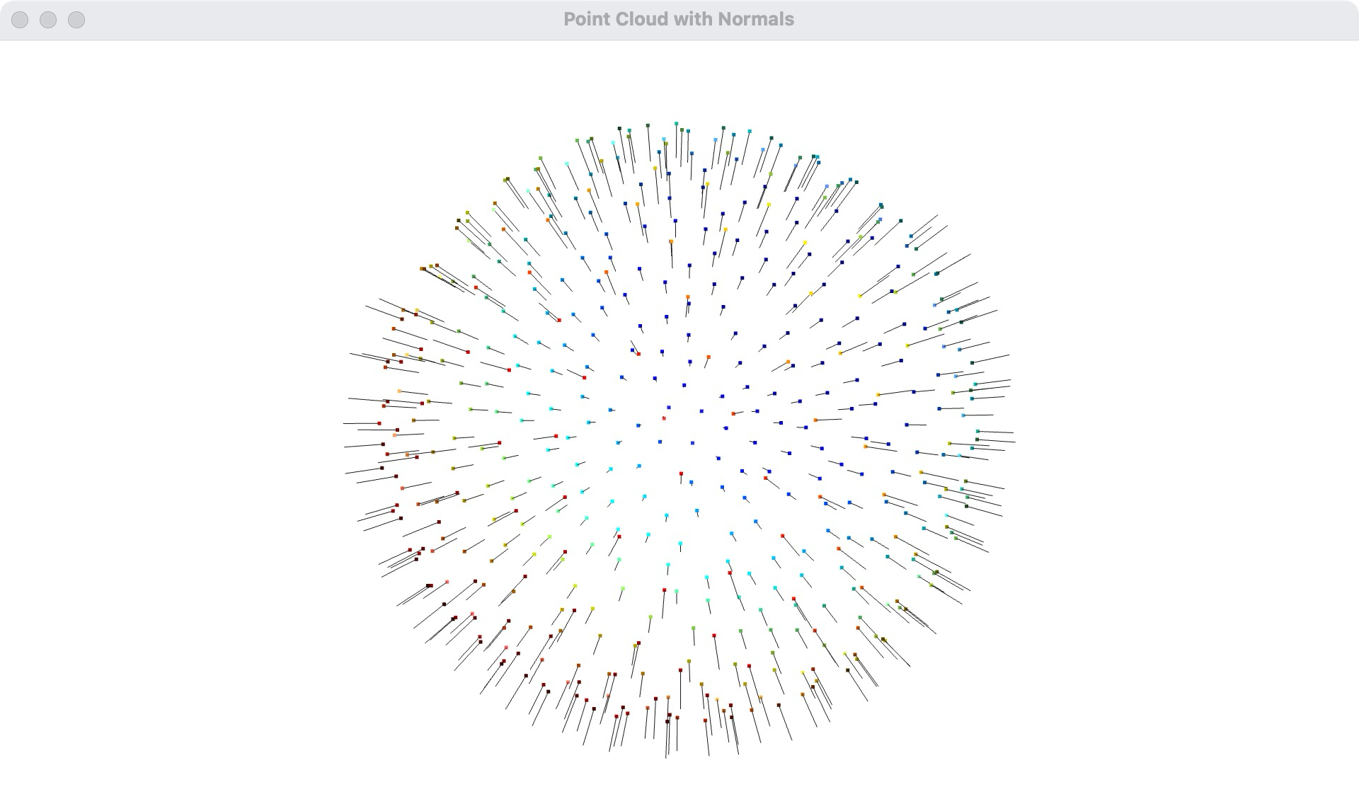 | 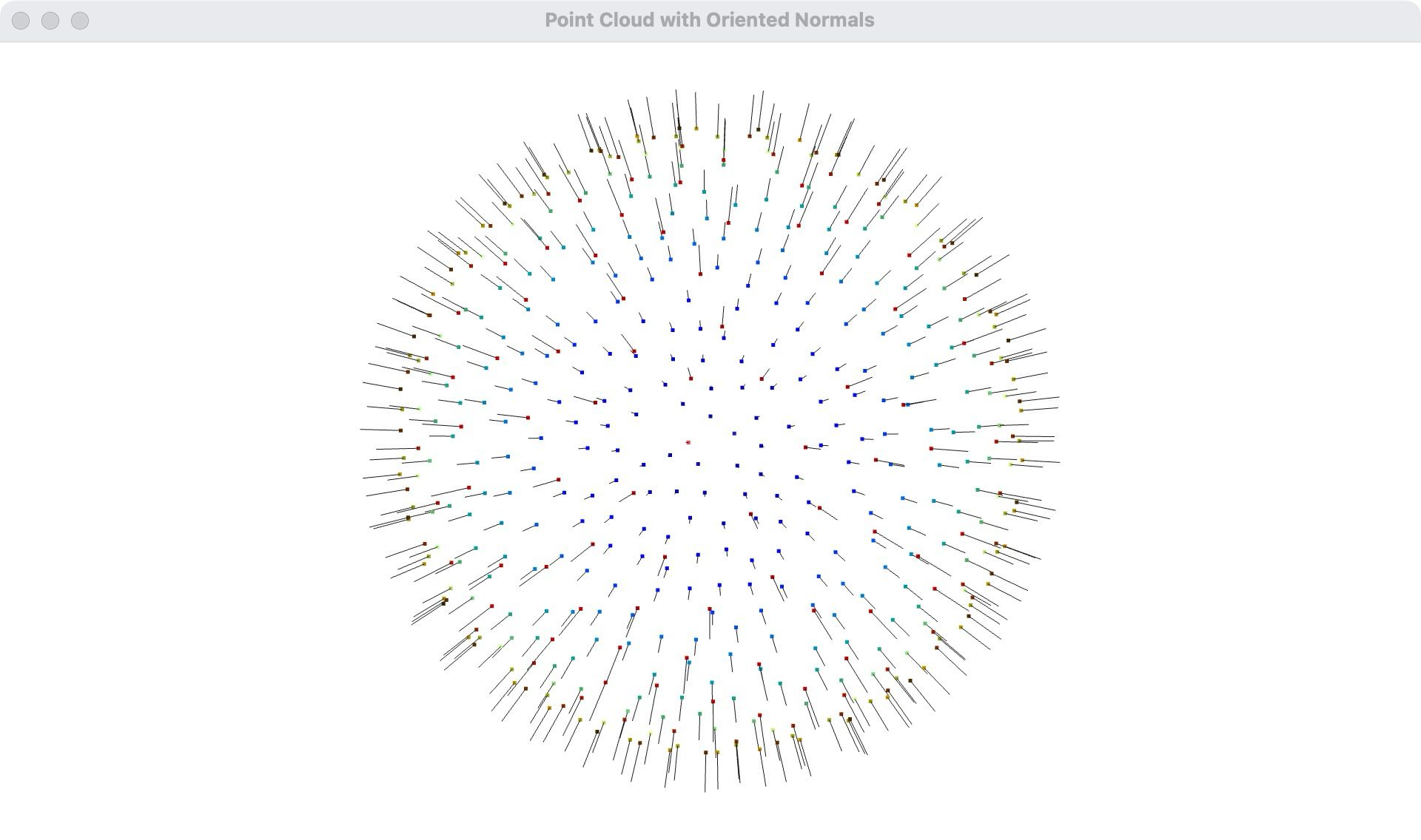 |
通过 estimate_normals 和 orient_normals_consistent_tangent_plane 方法,你可以估计点云的法线并使其方向一致。这对于后续的点云处理和分析(如表面重建、配准等)非常重要。
10. 点云配准
Open3D 提供了多种点云配准方法,主要包括以下几种:
ICP (Iterative Closest Point) 配准:这是最常用的点云配准方法之一,通过迭代地最小化两组点云之间的距离来实现配准。
Colored ICP 配准:这是对传统 ICP 的改进,除了几何距离外,还考虑了颜色信息来进行配准。
Global Registration (全局配准):用于初始配准,通常在没有初始对齐的情况下使用。包括 RANSAC-based 和 Fast Global Registration (FGR) 方法。
Multiway Registration (多路配准):用于将多个点云配准到一个共同的参考框架中。
下面是每种方法的说明和案例:
10.1 ICP 配准
说明:通过迭代地最小化两组点云之间的距离来实现配准。
案例:
import open3d as o3d
import numpy as np

def create_colored_point_cloud(color):
    """创建并上色的球体点云"""
    pcd = o3d.geometry.TriangleMesh.create_sphere(radius=1.0).sample_points_uniformly(number_of_points=1000)
    pcd.paint_uniform_color(color)
    return pcd

def visualize_point_clouds(pcd1, pcd2, window_name):
    """可视化点云"""
    o3d.visualization.draw_geometries([pcd1, pcd2], window_name=window_name)

# 生成并上色两个相似的点云
pcd1 = create_colored_point_cloud([1, 0, 0])  # 红色
pcd2 = create_colored_point_cloud([0, 1, 0])  # 绿色

# 对第二个点云进行初始变换
initial_transformation = np.array([[0.862, 0.011, -0.507, 0.5],
                                   [-0.139, 0.967, -0.215, 0.7],
                                   [0.487, 0.255, 0.835, -1.4],
                                   [0.0, 0.0, 0.0, 1.0]])
pcd2.transform(initial_transformation)

# 可视化初始点云
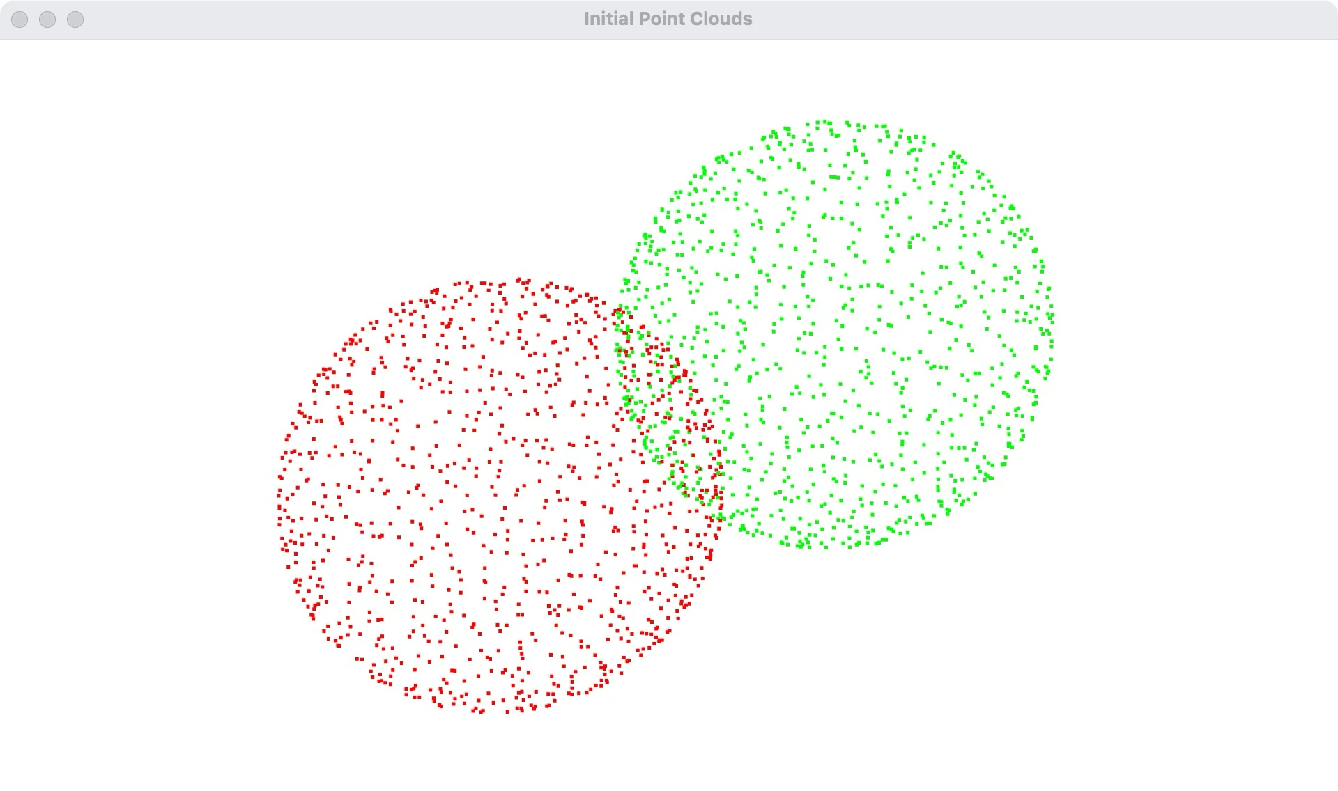
visualize_point_clouds(pcd1, pcd2, "Initial Point Clouds")

# 使用 ICP 进行配准
threshold = 0.7  # 增加阈值
trans_init = np.eye(4)
reg_p2p = o3d.pipelines.registration.registration_icp(
    pcd1, pcd2, threshold, trans_init,
    o3d.pipelines.registration.TransformationEstimationPointToPoint()
)

# 打印配准信息
print("ICP converged:", reg_p2p.inlier_rmse < threshold)
print("Fitness:", reg_p2p.fitness)
print("Inlier RMSE:", reg_p2p.inlier_rmse)
print("Transformation matrix:")
print(reg_p2p.transformation)

# 计算逆矩阵
inverse_transformation = np.linalg.inv(reg_p2p.transformation)

# 应用逆矩阵到第二个点云
pcd2.transform(inverse_transformation)

# 可视化配准后的点云
visualize_point_clouds(pcd1, pcd2, "Aligned Point Clouds")| 原始点云 | 配准点云 |
|---|---|
 | 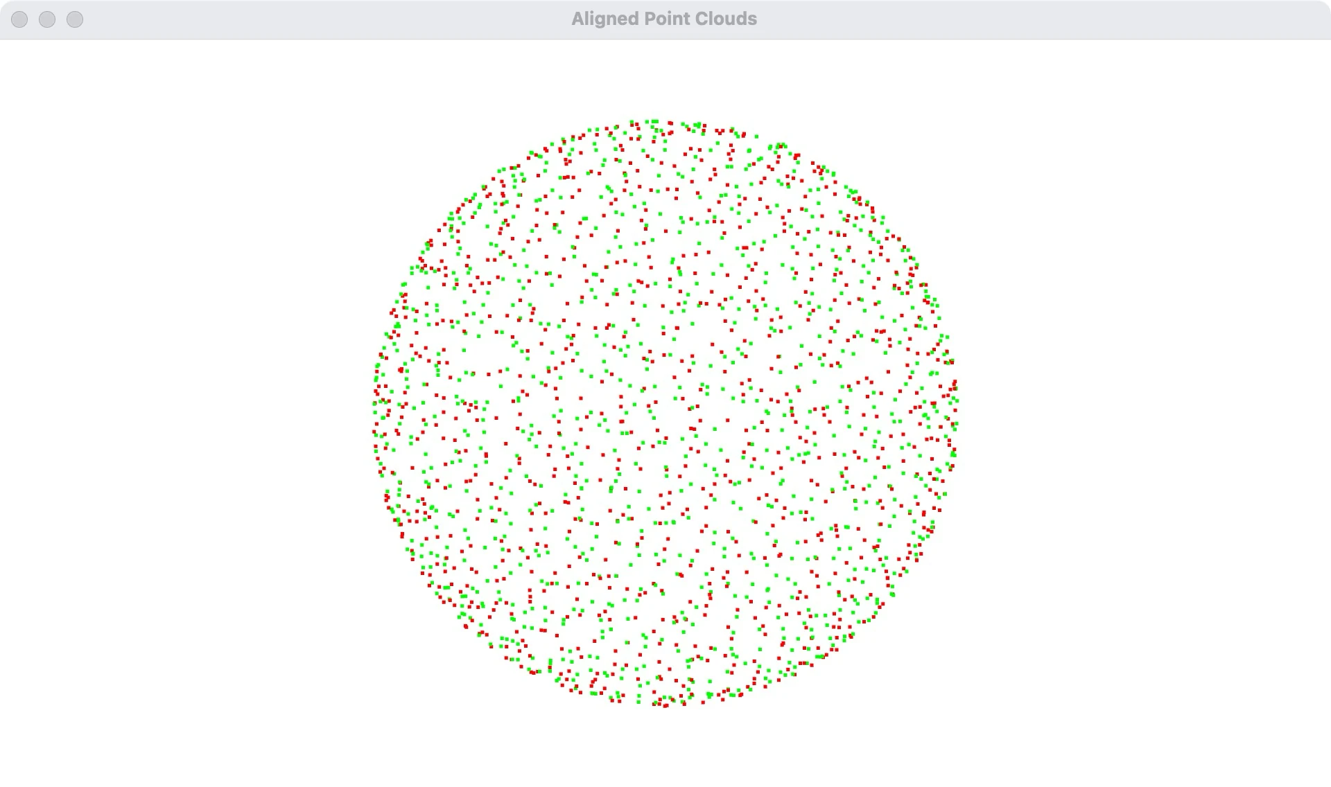 |
10.2 Colored ICP 配准
说明:Colored ICP 结合几何与颜色信息。下例保留球体作为 API 演示,但均匀颜色没有提供额外颜色梯度,球体几何又有旋转对称性,因此不能用它验证完整姿态恢复或 Colored ICP 的精度优势。实际测试应换为有纹理、非对称、尺度一致且重叠充分的数据,并与已知变换比较。
import open3d as o3d
import numpy as np

def create_colored_sphere(radius, color, density=1000):
    mesh = o3d.geometry.TriangleMesh.create_sphere(radius=radius)
    pcd = mesh.sample_points_poisson_disk(number_of_points=density)
    pcd.paint_uniform_color(color)
    return pcd

def estimate_normals(pcd, radius=0.1, max_nn=30):
    pcd.estimate_normals(search_param=o3d.geometry.KDTreeSearchParamHybrid(radius=radius, max_nn=max_nn))

def execute_colored_icp(source, target, max_correspondence_distance, initial_transformation):
    criteria = o3d.pipelines.registration.ICPConvergenceCriteria(
        relative_fitness=1e-3,
        relative_rmse=1e-3,
        max_iteration=500)
    result = o3d.pipelines.registration.registration_colored_icp(
        source, target, max_correspondence_distance, initial_transformation,
        o3d.pipelines.registration.TransformationEstimationForColoredICP(),
        criteria)
    return result

# 创建两个绿色的球体
sphere1 = create_colored_sphere(1.0, [0, 1, 0], density=1000)
sphere2 = create_colored_sphere(1.0, [0, 1, 0], density=1000)

# 对第二个球体进行变换
transformation = np.array([[0.862, 0.011, -0.507, 0.5],
                           [-0.139, 0.967, -0.215, 0.7],
                           [0.487, 0.255, 0.835, -1.4],
                           [0.0, 0.0, 0.0, 1.0]])
sphere2.transform(transformation)

# 估算法线
estimate_normals(sphere1)
estimate_normals(sphere2)

# 可视化配准前的点云
print("配准前的点云:")
o3d.visualization.draw_geometries([sphere1, sphere2], window_name="Before Registration")

# 使用彩色ICP进行配准
max_correspondence_distance = 5.0  # 增大最大对应点距离
initial_transformation = np.identity(4)
result_colored_icp = execute_colored_icp(sphere1, sphere2, max_correspondence_distance, initial_transformation)

# 应用变换到第一个球体点云
sphere1.transform(result_colored_icp.transformation)

# 可视化配准后的点云
print("配准后的点云:")
o3d.visualization.draw_geometries([sphere1, sphere2], window_name="After Registration")- 代码说明:
- 创建彩色球体:使用
create_colored_sphere函数创建两个绿色的球体。 - 对第二个球体进行变换:对第二个球体进行随机变换。
- 估算法线:计算球体点云的法线。
- 可视化配准前的点云:在配准前显示两个球体点云。
- 使用彩色ICP进行配准:使用彩色ICP算法进行配准。
- 应用变换到第一个球体点云:将配准结果应用到第一个球体点云。
- 可视化配准后的点云:在配准后显示两个球体点云。
| 原始点云 | 配准点云 |
|---|---|
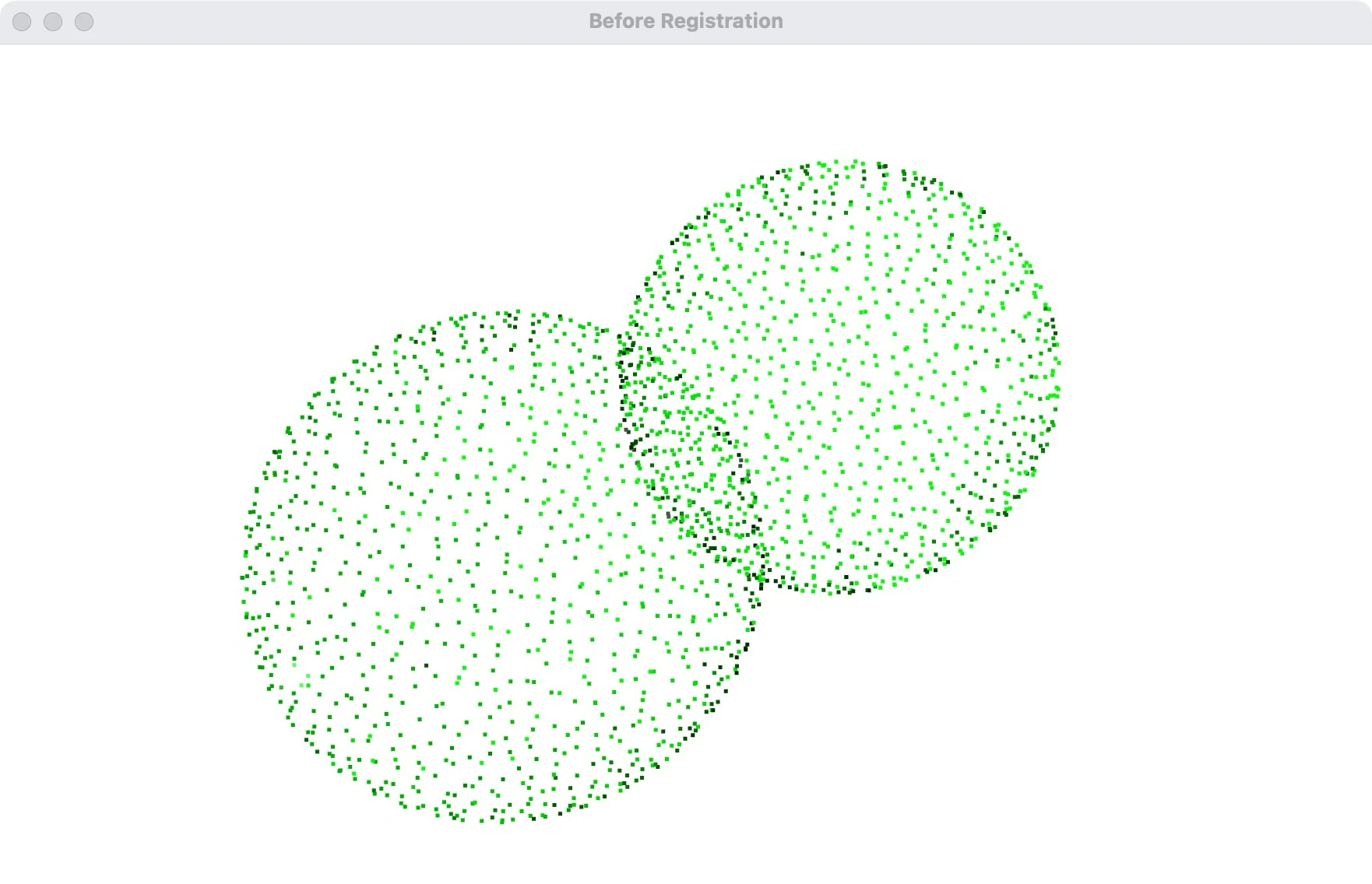 | 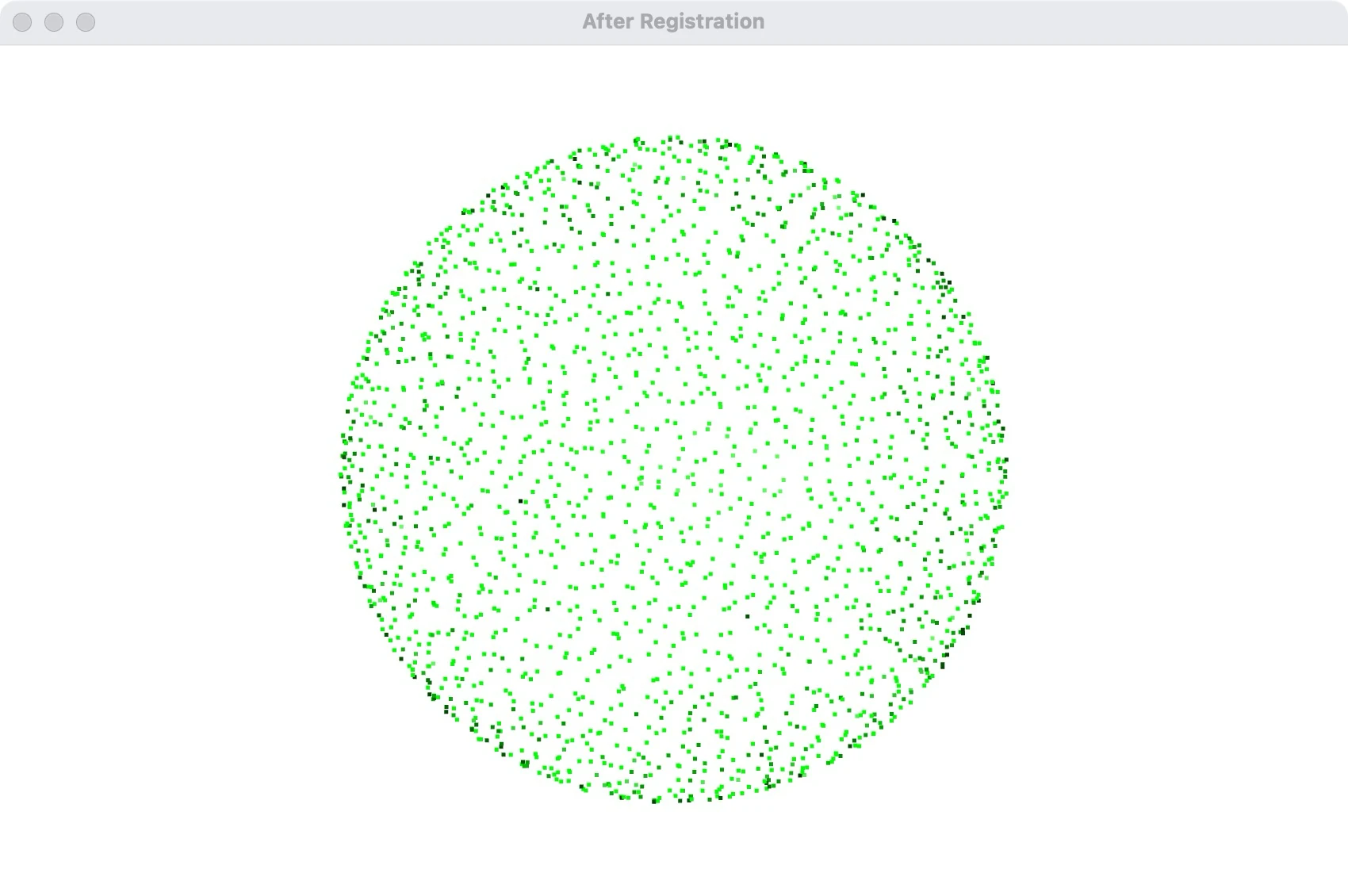 |
10.3 全局配准
说明:用于初始配准,通常在没有初始对齐的情况下使用。
下面是包含配准前后可视化的示例;随机几何上的匹配不保证成功,应检查 fitness、inlier_rmse 和已知变换误差:
import open3d as o3d
import numpy as np

# 生成点云数据
def generate_point_cloud():
    # 创建一个球体点云
    mesh = o3d.geometry.TriangleMesh.create_sphere(radius=1.0)
    pcd = mesh.sample_points_poisson_disk(number_of_points=500)
    return pcd

# 生成源点云和目标点云
source = generate_point_cloud()
target = generate_point_cloud()

# 对目标点云进行随机变换
transformation = np.array([[0.862, 0.011, -0.507, 0.5],
                           [-0.139, 0.967, -0.215, 0.7],
                           [0.487, 0.255, 0.835, -1.4],
                           [0.0, 0.0, 0.0, 1.0]])
target.transform(transformation)

# 下采样点云
voxel_size = 0.05
source_down = source.voxel_down_sample(voxel_size)
target_down = target.voxel_down_sample(voxel_size)

# 估计法线
source_down.estimate_normals(search_param=o3d.geometry.KDTreeSearchParamHybrid(radius=0.1, max_nn=30))
target_down.estimate_normals(search_param=o3d.geometry.KDTreeSearchParamHybrid(radius=0.1, max_nn=30))

# 计算FPFH特征
source_fpfh = o3d.pipelines.registration.compute_fpfh_feature(
    source_down,
    o3d.geometry.KDTreeSearchParamHybrid(radius=0.25, max_nn=100))
target_fpfh = o3d.pipelines.registration.compute_fpfh_feature(
    target_down,
    o3d.geometry.KDTreeSearchParamHybrid(radius=0.25, max_nn=100))

# 使用RANSAC进行全局配准
result_ransac = o3d.pipelines.registration.registration_ransac_based_on_feature_matching(
    source_down, target_down, source_fpfh, target_fpfh,
    mutual_filter=True,
    max_correspondence_distance=0.15,
    estimation_method=o3d.pipelines.registration.TransformationEstimationPointToPoint(False),
    ransac_n=4,
    checkers=[o3d.pipelines.registration.CorrespondenceCheckerBasedOnEdgeLength(0.9),
              o3d.pipelines.registration.CorrespondenceCheckerBasedOnDistance(0.15)],
    criteria=o3d.pipelines.registration.RANSACConvergenceCriteria(4000000, 500))

print(result_ransac)

# 可视化配准前的点云
source_temp = source_down.transform(np.identity(4))  # 恢复原始位置
o3d.visualization.draw_geometries([source_temp, target_down], window_name="配准前")

# 可视化配准后的点云
source_temp = source_down.transform(result_ransac.transformation)
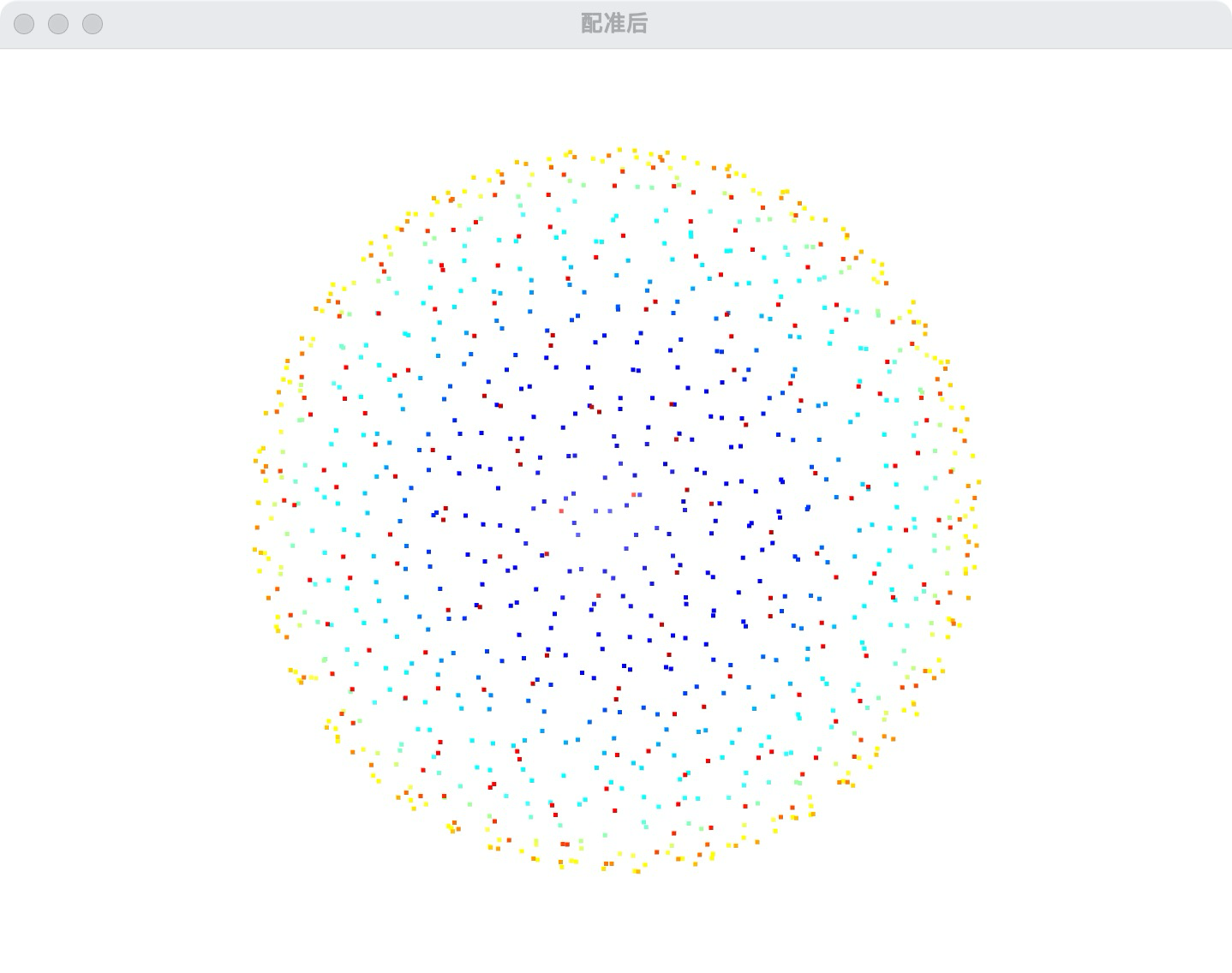
o3d.visualization.draw_geometries([source_temp, target_down], window_name="配准后")- 代码说明:
- 生成点云数据:创建一个球体点云,并对目标点云进行随机变换。
- 下采样点云:对点云进行体素下采样,以减少计算量。
- 估计法线:计算点云的法线。
- 计算FPFH特征:计算快速点特征直方图(FPFH)特征。
- 使用RANSAC进行全局配准:使用 RANSAC 算法基于特征匹配进行全局配准。
- 可视化配准前的点云:在配准前显示源点云和目标点云。
- 可视化配准后的点云:在配准后显示源点云和目标点云。
| 初始点云 | 配准点云 |
|---|
| 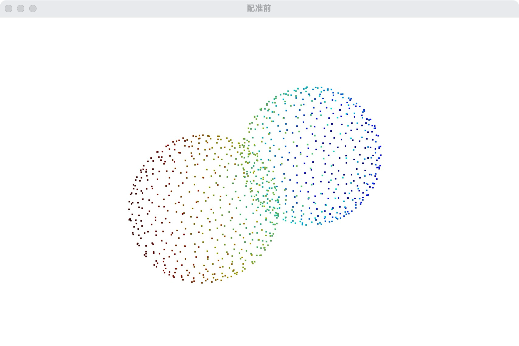 |
|  |
|
10.4 多路配准
说明:用于将多个点云配准到一个共同的参考框架中。
import open3d as o3d
import numpy as np

def create_colored_sphere(radius, color, density=1000):
    mesh = o3d.geometry.TriangleMesh.create_sphere(radius=radius)
    pcd = mesh.sample_points_poisson_disk(number_of_points=density)
    pcd.paint_uniform_color(color)
    return pcd

def preprocess_point_cloud(pcd, voxel_size):
    pcd_down = pcd.voxel_down_sample(voxel_size)
    radius_normal = voxel_size * 2
    pcd_down.estimate_normals(o3d.geometry.KDTreeSearchParamHybrid(radius=radius_normal, max_nn=30))
    radius_feature = voxel_size * 5
    pcd_fpfh = o3d.pipelines.registration.compute_fpfh_feature(
        pcd_down,
        o3d.geometry.KDTreeSearchParamHybrid(radius=radius_feature, max_nn=100))
    return pcd_down, pcd_fpfh

def pairwise_registration(source, target, voxel_size):
    source_down, source_fpfh = preprocess_point_cloud(source, voxel_size)
    target_down, target_fpfh = preprocess_point_cloud(target, voxel_size)

    distance_threshold = voxel_size * 1.5
    result = o3d.pipelines.registration.registration_ransac_based_on_feature_matching(
        source_down, target_down, source_fpfh, target_fpfh, True,
        distance_threshold,
        o3d.pipelines.registration.TransformationEstimationPointToPoint(False),
        4, [
            o3d.pipelines.registration.CorrespondenceCheckerBasedOnEdgeLength(0.9),
            o3d.pipelines.registration.CorrespondenceCheckerBasedOnDistance(distance_threshold)
        ], o3d.pipelines.registration.RANSACConvergenceCriteria(4000000, 500))
    return result

def full_registration(pcds, voxel_size):
    pose_graph = o3d.pipelines.registration.PoseGraph()
    odometry = np.identity(4)
    pose_graph.nodes.append(o3d.pipelines.registration.PoseGraphNode(odometry))

    for source_id in range(len(pcds)):
        for target_id in range(source_id + 1, len(pcds)):
            result = pairwise_registration(pcds[source_id], pcds[target_id], voxel_size)
            trans = result.transformation
            information = o3d.pipelines.registration.get_information_matrix_from_point_clouds(
                pcds[source_id], pcds[target_id], voxel_size * 1.5, result.transformation)
            if target_id == source_id + 1:
                odometry = np.dot(trans, odometry)
                pose_graph.nodes.append(o3d.pipelines.registration.PoseGraphNode(np.linalg.inv(odometry)))
                pose_graph.edges.append(o3d.pipelines.registration.PoseGraphEdge(source_id, target_id, trans, information, uncertain=False))
            else:
                pose_graph.edges.append(o3d.pipelines.registration.PoseGraphEdge(source_id, target_id, trans, information, uncertain=True))
    return pose_graph

def run_global_optimization(pose_graph):
    option = o3d.pipelines.registration.GlobalOptimizationOption(
        max_correspondence_distance=0.02,
        edge_prune_threshold=0.25,
        reference_node=0)
    o3d.pipelines.registration.global_optimization(
        pose_graph,
        o3d.pipelines.registration.GlobalOptimizationLevenbergMarquardt(),
        o3d.pipelines.registration.GlobalOptimizationConvergenceCriteria(),
        option)

def merge_point_clouds(pcds, pose_graph):
    pcd_combined = o3d.geometry.PointCloud()
    for point_id in range(len(pcds)):
        pcd_transformed = pcds[point_id].transform(pose_graph.nodes[point_id].pose)
        pcd_combined += pcd_transformed
    return pcd_combined

# 从同一非对称物体采样,不能用不同半径球体验证刚性配准
import copy
mesh = o3d.geometry.TriangleMesh.create_box(width=1.0, height=0.6, depth=0.3)
sphere1 = mesh.sample_points_uniformly(number_of_points=2000)
sphere2 = copy.deepcopy(sphere1)
sphere3 = copy.deepcopy(sphere1)
sphere1.paint_uniform_color([1, 0, 0])
sphere2.paint_uniform_color([0, 1, 0])
sphere3.paint_uniform_color([0, 0, 1])

# 对球体进行随机变换
transformation1 = np.array([[0.862, 0.011, -0.507, 0.5],
                            [-0.139, 0.967, -0.215, 0.7],
                            [0.487, 0.255, 0.835, -1.4],
                            [0.0, 0.0, 0.0, 1.0]])
sphere2.transform(transformation1)

transformation2 = np.array([[0.707, -0.707, 0.0, 1.0],
                            [0.707, 0.707, 0.0, 0.5],
                            [0.0, 0.0, 1.0, -0.5],
                            [0.0, 0.0, 0.0, 1.0]])
sphere3.transform(transformation2)

pcds = [sphere1, sphere2, sphere3]

# 设置体素大小
voxel_size = 0.05

# 可视化配准前的点云
print("配准前的点云")
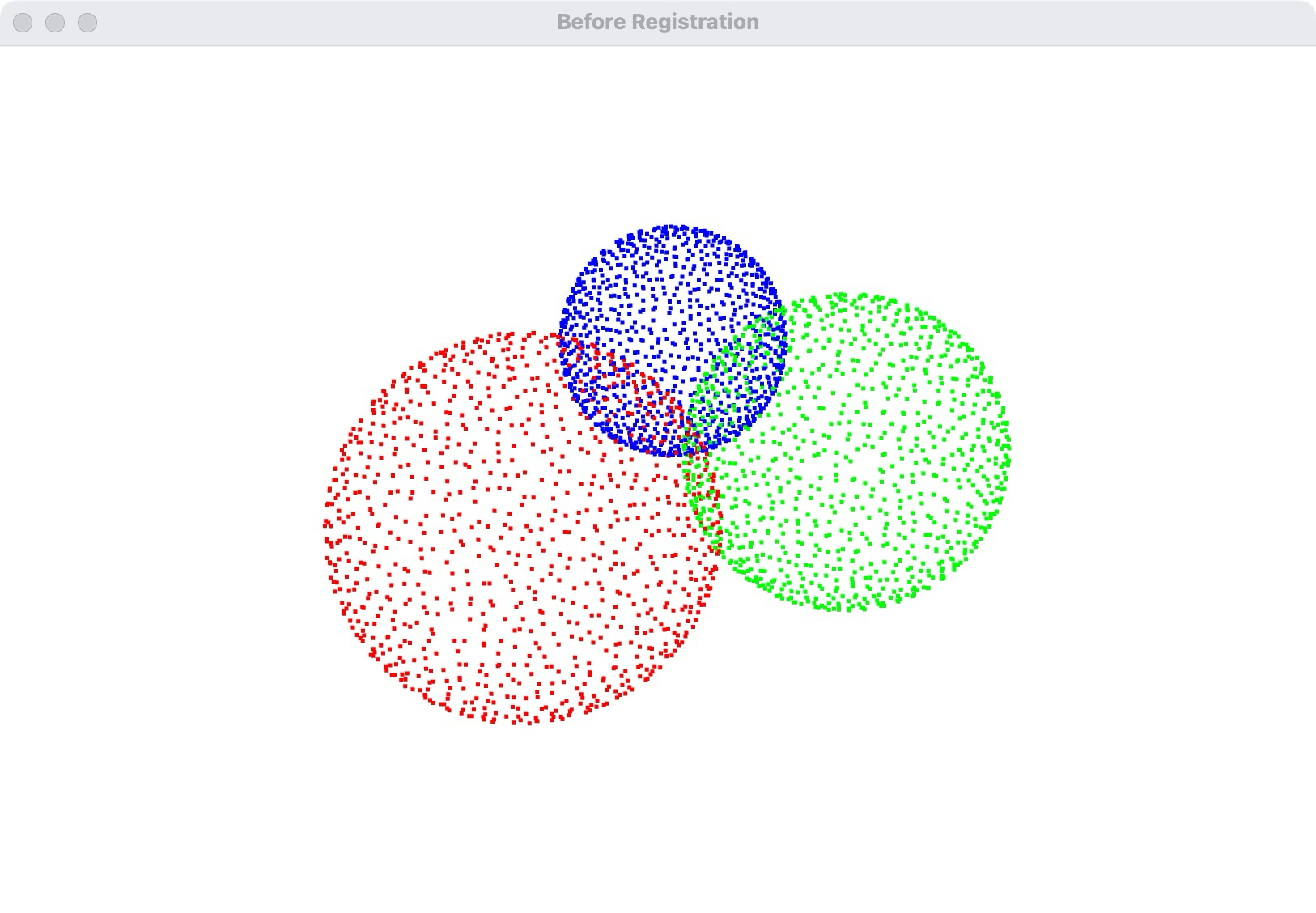
o3d.visualization.draw_geometries(pcds, window_name="Before Registration")

# 进行多路配准
pose_graph = full_registration(pcds, voxel_size)

# 运行全局优化
run_global_optimization(pose_graph)

# 合并点云
pcd_combined = merge_point_clouds(pcds, pose_graph)

# 可视化配准后的点云
print("配准后的点云")
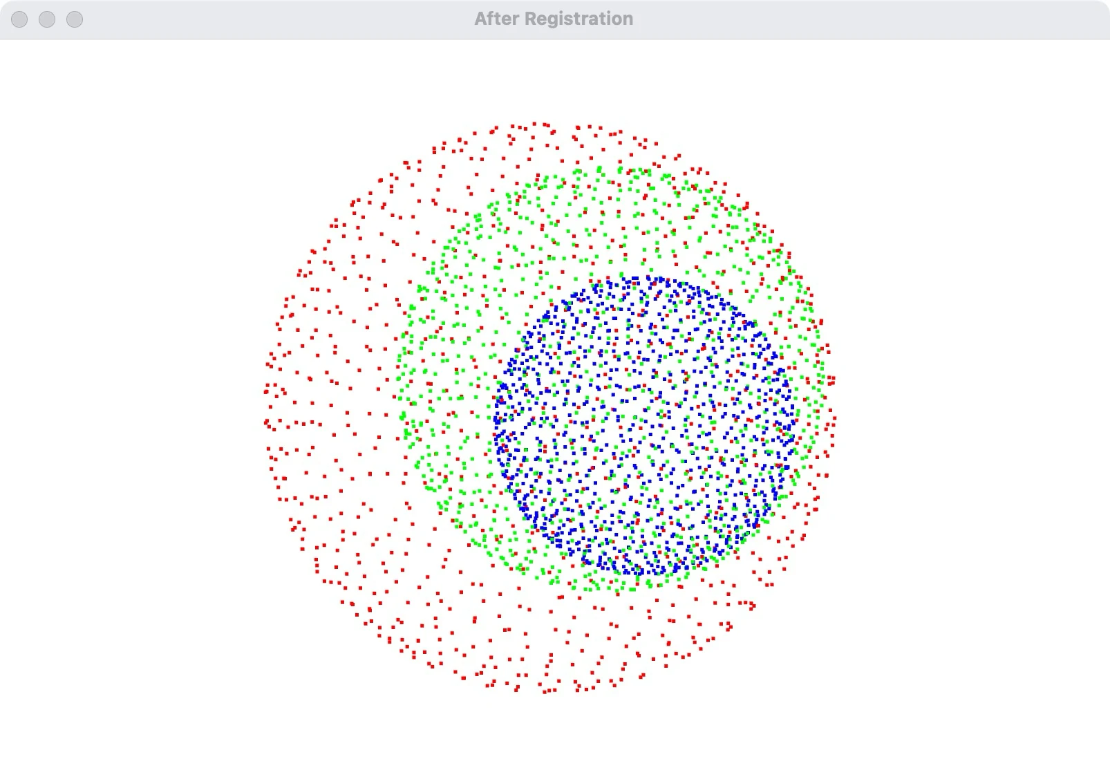
o3d.visualization.draw_geometries([pcd_combined], window_name="After Registration")- 代码说明:
- 创建彩色球体:从同一长方体生成三组等尺度点云;变量名为历史命名。原图是旧版示意,不作为修订代码的精度验证。
- 对球体进行变换:对第二个和第三个球体进行随机变换。
- 预处理点云:使用
preprocess_point_cloud函数对点云进行下采样和特征提取。 - 配对配准:使用
pairwise_registration函数对两个点云进行配对配准。 - 全局配准:使用
full_registration函数对所有点云进行全局配准,构建位姿图。 - 全局优化:使用
run_global_optimization函数对位姿图进行全局优化。 - 合并点云:使用
merge_point_clouds函数将所有点云合并到一个全局坐标系中。 - 可视化配准前的点云:使用 Open3D 的可视化工具显示配准前的点云。
- 可视化配准后的点云:使用 Open3D 的可视化工具显示配准后的点云。
| 原始点云 | 配准点云 |
|---|
|  |
|  |
|
这些案例展示了 Open3D 中不同点云配准方法的基本用法。
11. 点云表面重建
11.1 Alpha形状重建
Alpha形状重建是一种用于从点云数据生成三角网格的方法。它基于计算几何中的Alpha形状理论。Alpha形状是由Edelsbrunner等人在1983年提出的,它是Delaunay三角剖分的一个子集,用于描述点集的形状。
11.1.1 原理
Delaunay三角剖分:
- 首先,对点云进行Delaunay三角剖分。Delaunay三角剖分是一种将点集划分为一系列三角形的算法,具有最大化最小角的性质,避免了瘦长三角形。
Alpha球:
- 对于给定的参数α,定义一个半径为α的球(称为Alpha球)。Alpha球用于筛选Delaunay三角剖分中的三角形。
筛选三角形:
- 对于每个Delaunay三角剖分中的三角形,检查其外接圆的半径。如果外接圆的半径小于或等于α,则保留该三角形;否则,丢弃该三角形。
生成Alpha形状:
- 保留的三角形构成了Alpha形状。通过调整α的值,可以控制生成的形状的细节程度。较小的α值会生成更细致的形状,而较大的α值会生成更平滑的形状。
11.1.2 代码示例
以下是使用Open3D库进行Alpha形状重建的代码示例:
import open3d as o3d

# 读取点云
pcd = o3d.io.read_point_cloud("doll_1.ply")

# 估计法线
pcd.estimate_normals(search_param=o3d.geometry.KDTreeSearchParamHybrid(radius=0.1, max_nn=30))

# Alpha形状重建
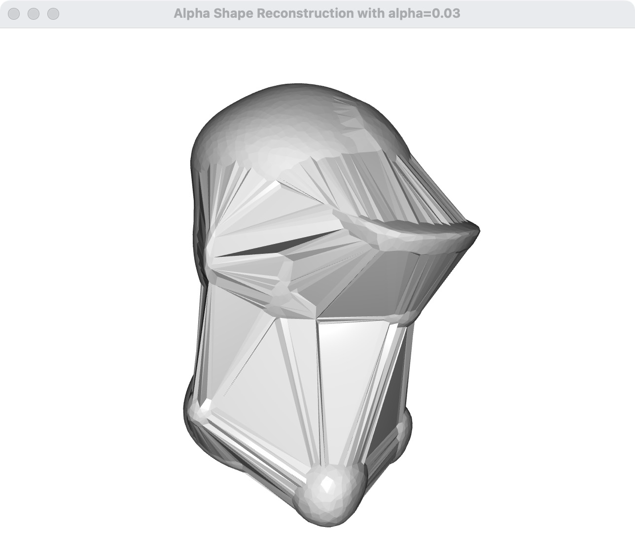
alpha = 0.03  # 调整alpha值
mesh_alpha = o3d.geometry.TriangleMesh.create_from_point_cloud_alpha_shape(pcd, alpha)

# 可视化Alpha形状重建结果
mesh_alpha.compute_vertex_normals()
o3d.visualization.draw_geometries([mesh_alpha], window_name=f"Alpha Shape Reconstruction with alpha={alpha}")
11.1.3 调整Alpha值
通过调整alpha值,可以生成不同细节程度的形状:
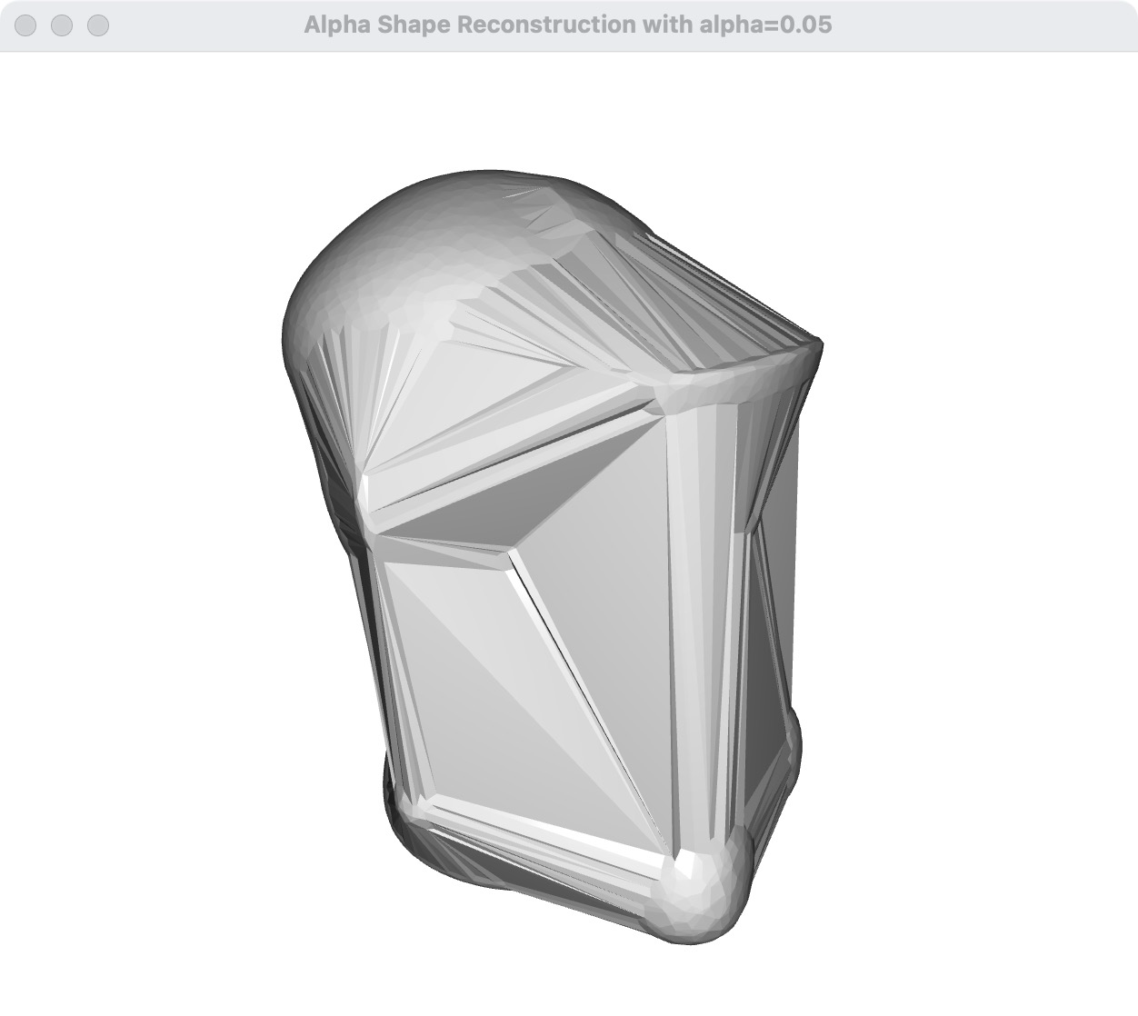
- 较小的 alpha:可能保留细结构,也可能断裂、产生孔洞或空结果。
- 较大的 alpha:连接更多区域,极限趋向凸包,不等同于普通平滑滤波。
11.1.4 总结
Alpha形状重建是一种有效的从点云数据生成三角网格的方法,通过调整alpha值,可以控制生成形状的细节程度。它在计算几何和计算机图形学中有广泛的应用。
import open3d as o3d

# 读取点云
pcd = o3d.io.read_point_cloud("doll_1.ply")

# 估计法线
pcd.estimate_normals(search_param=o3d.geometry.KDTreeSearchParamHybrid(radius=0.1, max_nn=30))

# 调整Alpha形状重建参数
print("调整Alpha形状重建参数...")
alphas = [0.01, 0.03, 0.05]
for alpha in alphas:
    mesh_alpha = o3d.geometry.TriangleMesh.create_from_point_cloud_alpha_shape(pcd, alpha)
    mesh_alpha.compute_vertex_normals()
    title = f"Alpha Shape Reconstruction with alpha={alpha}"
    print(title)
    o3d.visualization.draw_geometries([mesh_alpha], window_name=title)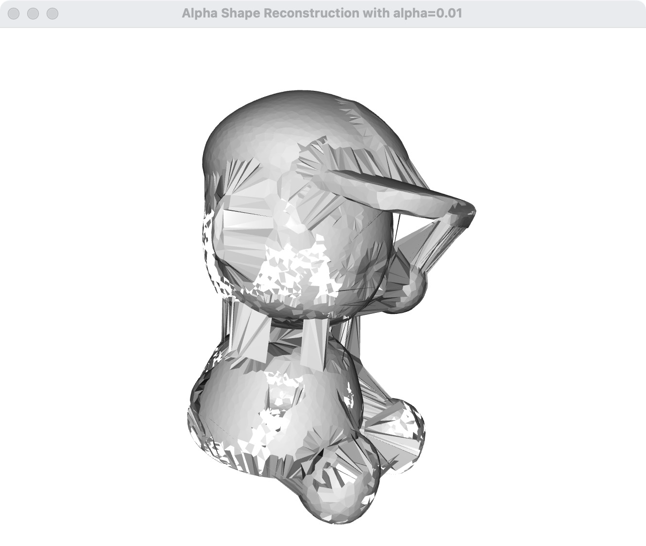
11.2 泊松重建
输入需要方向一致的法线;estimate_normals 本身不保证全局朝向正确。重建结果可能在低密度区域外推,需结合返回的 density、观测边界和任务需求裁剪,而不是将输出整体视为真实观测表面。
泊松重建(Poisson Surface Reconstruction)是一种从点云数据生成平滑三角网格的方法。它基于泊松方程,通过全局优化的方法生成表面,能够有效处理噪声和不完整的点云数据。
11.2.1 原理
法线估计:
- 首先,从点云数据中估计每个点的法线方向。这一步通常使用邻域搜索算法,如KD树搜索。
泊松方程: 泊松重建的核心是求解泊松方程。泊松方程是一种偏微分方程,形式为:
其中, 是一个向量场, 是一个标量场。在泊松重建中, 是由点云的法线生成的向量场, 是点云的散度。
构建八叉树:
- 为了高效地求解泊松方程,使用八叉树(Octree)对点云进行分层表示。八叉树将空间递归地划分为八个子空间,直到达到指定的深度。
求解泊松方程:
- 在八叉树的每个节点上,求解泊松方程。通过最小二乘法或其他数值方法,计算出每个节点的标量场值。
提取等值面:
- 使用Marching Cubes算法从标量场中提取等值面,生成三角网格。等值面是标量场中具有相同值的点的集合。
平滑和优化:
- 对生成的三角网格进行平滑和优化,以去除噪声和不规则性,生成最终的平滑表面。
11.2.2 代码示例
以下是使用Open3D库进行泊松重建的代码示例:
import open3d as o3d

# 读取点云
pcd = o3d.io.read_point_cloud("doll_1.ply")

# 估计法线
pcd.estimate_normals(search_param=o3d.geometry.KDTreeSearchParamHybrid(radius=0.1, max_nn=30))

# 泊松重建
depth = 9  # 调整深度参数
mesh_poisson, densities = o3d.geometry.TriangleMesh.create_from_point_cloud_poisson(pcd, depth=depth)

# 可视化泊松重建结果
mesh_poisson.compute_vertex_normals()
o3d.visualization.draw_geometries([mesh_poisson], window_name=f"Poisson Reconstruction with depth={depth}")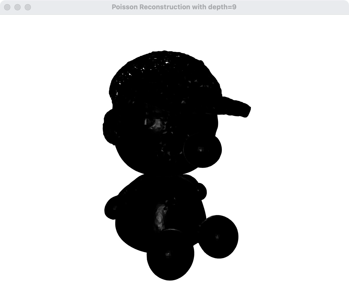
11.2.3 调整深度参数
通过调整深度参数,可以控制生成的网格的细节程度:
- 较小的深度值:生成的网格较粗糙,计算速度较快。
- 较大的深度值:生成的网格较细致,计算速度较慢。
11.2.4 总结
泊松重建是一种从点云数据生成平滑三角网格的有效方法。它通过求解泊松方程,能够处理噪声和不完整的点云数据,生成高质量的表面。通过调整深度参数,可以控制生成网格的细节程度。
12. 最小包围盒
使用Open3D计算点云的包围盒可以通过以下两种方式:轴对齐包围盒(Axis-Aligned Bounding Box, AABB)和有向包围盒(Oriented Bounding Box, OBB)。 下面是一个示例代码,展示如何计算和可视化这两种包围盒。
- 示例代码
import open3d as o3d

# 读取点云
pcd = o3d.io.read_point_cloud("doll_1.ply")

# 计算轴对齐包围盒(AABB)
aabb = pcd.get_axis_aligned_bounding_box()

# 计算有向包围盒(OBB)
obb = pcd.get_oriented_bounding_box()

# 设置包围盒的颜色
aabb.color = (1, 0, 0)  # 红色
obb.color = (0, 1, 0)   # 绿色

# 可视化点云和包围盒
o3d.visualization.draw_geometries([pcd, aabb, obb], window_name="Bounding Boxes")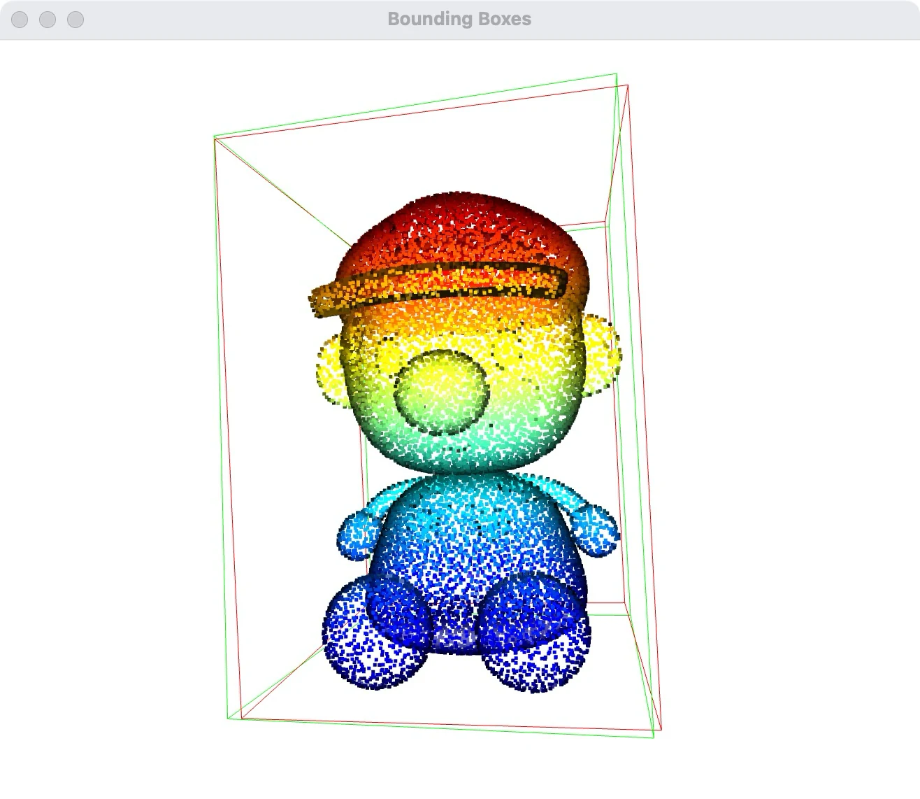
- 说明
读取点云:
- 使用
o3d.io.read_point_cloud函数读取点云数据。
- 使用
计算轴对齐包围盒(AABB):
- 使用
pcd.get_axis_aligned_bounding_box()方法计算点云的轴对齐包围盒。AABB是一个与坐标轴对齐的最小包围盒。
- 使用
计算有向包围盒(OBB):
- 使用
pcd.get_oriented_bounding_box()方法计算点云的有向包围盒。该接口通常基于 PCA 计算近似 OBB,不保证全局最小体积;精确/更紧的包围盒需核对版本提供的相应接口。
- 使用
设置包围盒的颜色:
- 通过设置
color属性来改变包围盒的颜色,以便在可视化时区分不同的包围盒。
- 通过设置
可视化点云和包围盒:
- 使用
o3d.visualization.draw_geometries函数同时可视化点云和包围盒。
- 使用
- 总结
通过上述代码,可以使用Open3D计算点云的轴对齐包围盒和有向包围盒,并进行可视化。这对于点云数据的分析和处理非常有用。
13. 凸包
使用Open3D计算点云的凸包可以通过 compute_convex_hull 方法来实现。
以下是一个示例代码,展示如何计算和可视化点云的凸包。
- 示例代码
import open3d as o3d

# 读取点云
pcd = o3d.io.read_point_cloud("doll_1.ply")

# 计算凸包
hull, _ = pcd.compute_convex_hull()

# 设置凸包的颜色
hull.paint_uniform_color([1, 0, 0])  # 红色

# 可视化点云和凸包
o3d.visualization.draw_geometries([pcd, hull], window_name="Convex Hull")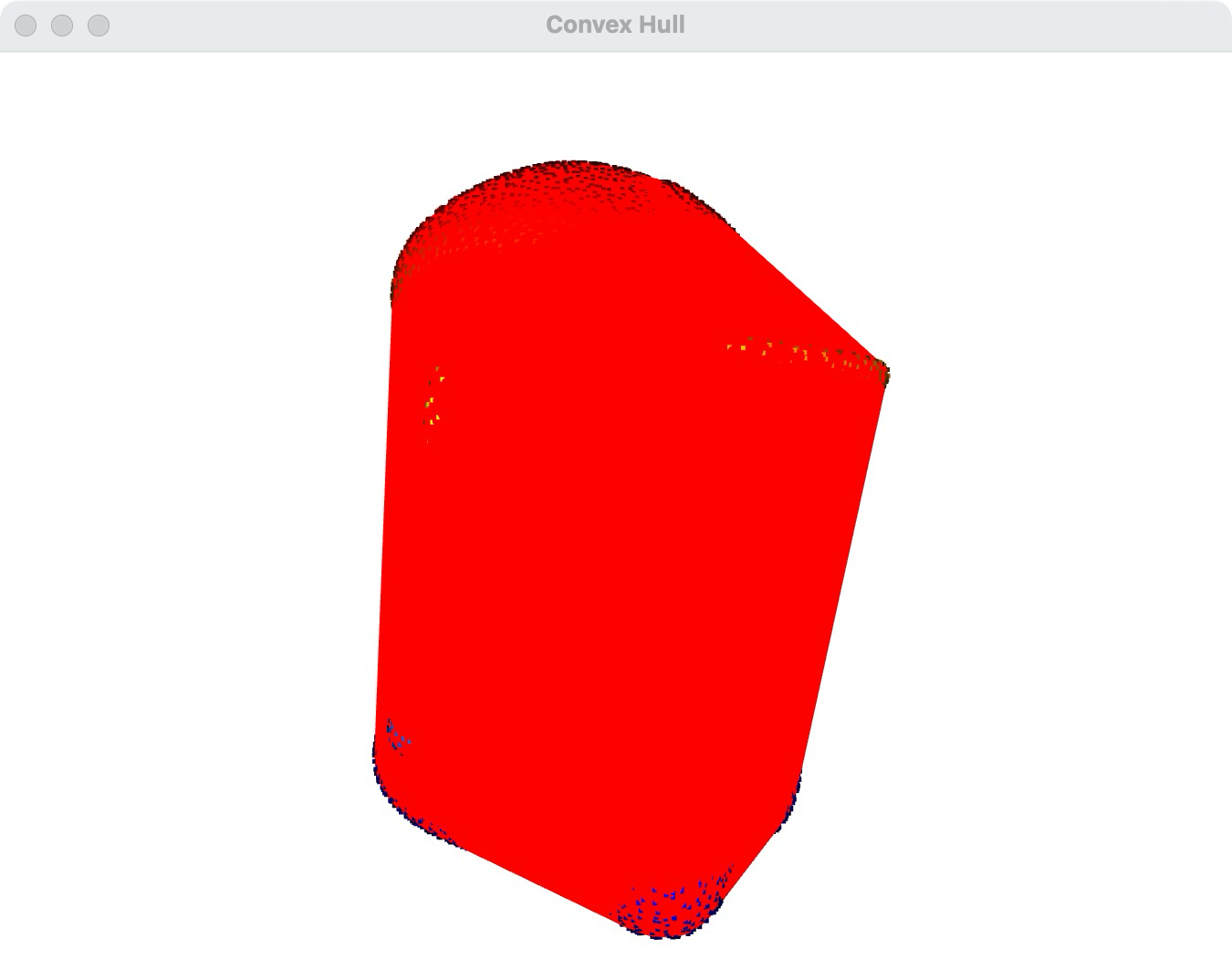
- 说明
读取点云:
- 使用
o3d.io.read_point_cloud函数读取点云数据。
- 使用
计算凸包:
- 使用
pcd.compute_convex_hull()方法计算点云的凸包。该方法返回一个三角网格表示的凸包和一个索引数组(这里我们只关心凸包)。
- 使用
设置凸包的颜色:
- 使用
hull.paint_uniform_color([1, 0, 0])方法将凸包的颜色设置为红色,以便在可视化时区分凸包和点云。
- 使用
可视化点云和凸包:
- 使用
o3d.visualization.draw_geometries函数同时可视化点云和凸包。
- 使用
总结
- 通过上述代码,可以使用Open3D计算点云的凸包,并进行可视化。这对于点云数据的分析和处理非常有用,特别是在需要了解点云的外部形状时。
14. 体素化
下面使用 VoxelGrid.create_from_point_cloud 建立占用体素。它与返回平均点位置的 voxel_down_sample 不同,不应把占用体素中心和原始点的重心混为一谈。
以下是一个示例代码,展示如何对点云进行体素化处理并进行可视化。
- 示例代码
import open3d as o3d

# 读取点云
pcd = o3d.io.read_point_cloud("doll_1.ply")

# 设置体素大小
voxel_size = 0.05

# 进行体素化
voxel_grid = o3d.geometry.VoxelGrid.create_from_point_cloud(pcd, voxel_size=voxel_size)

# 可视化原始点云和体素化后的点云
o3d.visualization.draw_geometries([pcd], window_name="Original Point Cloud")
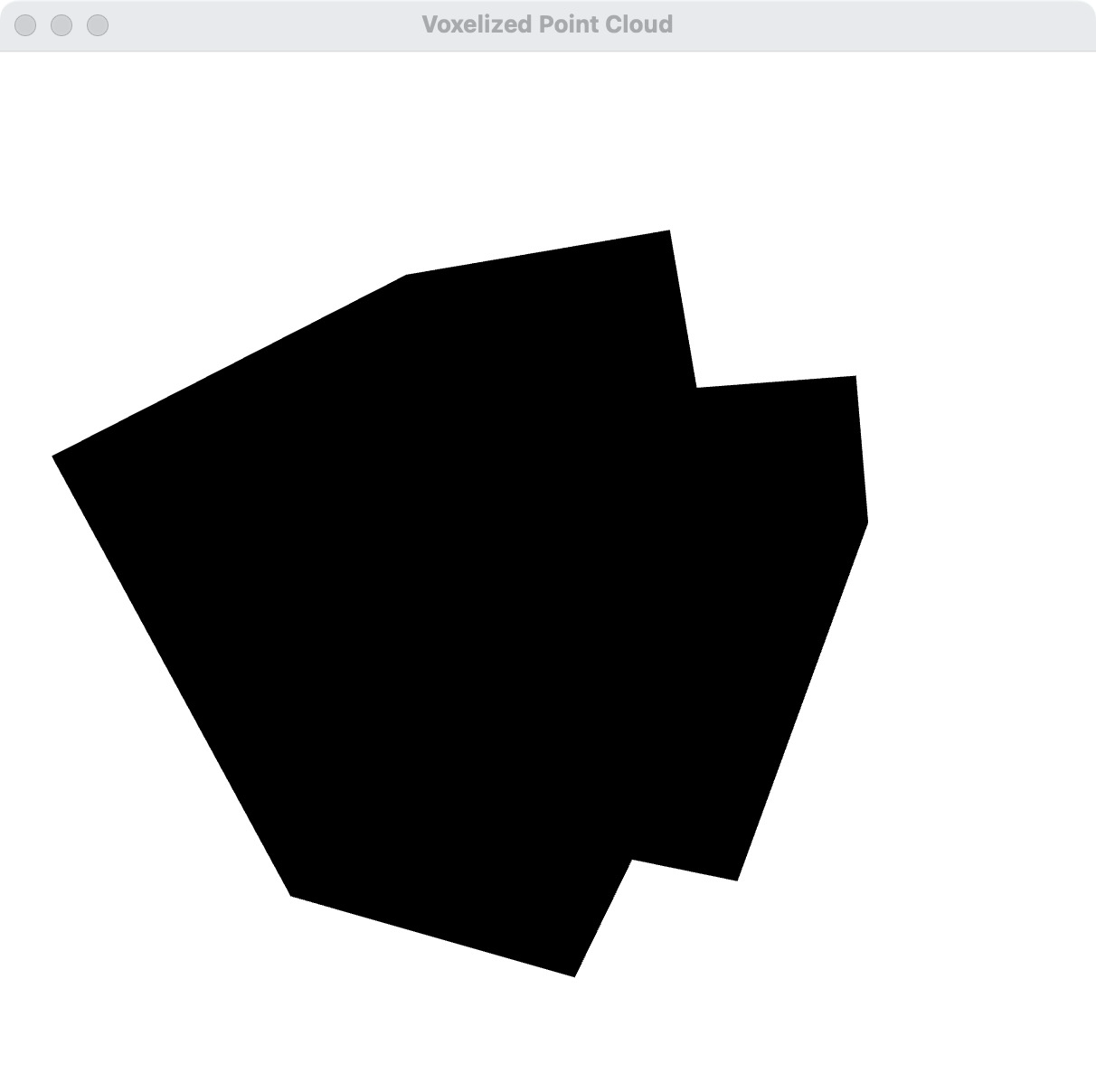
o3d.visualization.draw_geometries([voxel_grid], window_name="Voxelized Point Cloud")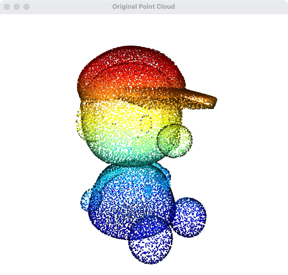
- 说明
读取点云:
- 使用
o3d.io.read_point_cloud函数读取点云数据。
- 使用
设置体素大小:
- 定义体素的大小(例如
voxel_size = 0.05),该值决定了每个体素的边长。
- 定义体素的大小(例如
进行体素化:
- 使用
o3d.geometry.VoxelGrid.create_from_point_cloud(pcd, voxel_size=voxel_size)方法对点云进行体素化处理。该方法返回一个VoxelGrid对象,表示体素化后的点云。
- 使用
可视化原始点云和体素化后的点云:
- 使用
o3d.visualization.draw_geometries函数分别可视化原始点云和体素化后的点云。
- 使用
总结
- 通过上述代码,可以使用Open3D对点云进行体素化处理,并进行可视化。体素化处理可以有效地减少点云数据的数量,同时保留点云的整体结构,对于点云数据的分析和处理非常有用。
阅读自测与验收
- 对滤波前后点数、法线、包围盒和坐标单位做数值检查;可视化颜色或视角变化不等于几何处理成功。
- 在已知刚体变换的点云上检验配准,同时报告 fitness、RMSE 与变换误差;对称物体尤其不能仅凭视觉重合判断唯一解。